|
|
|
8:12 |
|
|
transcript
|
1:45 |
Hello and welcome to my course Excel, to Python. We're so excited to have you here. Have you been using excel a lot in your data work and feel like there has to be a better way? Or maybe you have heard the Python is a good language to learn for data science and you will see how you could apply these concepts to your job. If so, then you're in the right place. We're going to have a lot of fun and get many ideas for using Python as an alternative to the task. You might try to use Excel for today before taking this course. You should have some experience with Python. If you are not comfortable with the basic concepts of Python. Then should look at our other course Python "Jump Start by Building 10 Applications" or "Python for the Absolute Beginner. In this course, you will learn how to set up and use a robust Python environment form, organized and repeatable process that could be used to replace many of the cumbersome tasks you use excel for today. The majority of the code in this class will be using the "Pandas Library" we will take a unique way to teach this powerful library by showing you examples and excel and translating them to the pandas version. You will start to learn more about pandas and understand when it will be a good alternative to your current Excel solutions. By the end of this course, you will understand how to incorporate Python into your daily analysis workflow. You will also find ways to streamline and automate many of the boring and repetitive tasks use typically do in Excel. Michael Kennedy frequently says that knowing Python is like having a superpower. I think there's a great analogy, and I suspect that by the time you finish this course, you will have many ideas for how you can take this knowledge back to your job, improve a tedious process and look like a super hero for saving your organization time
|
|
|
transcript
|
1:28 |
before we go into Python, let's talk a little about some of the challenges with Excel. Let's take a look at one really big financial disaster that had excel as a part of the problem. Many of you may have heard about the massive trading losses that JP Morgan and Chase experienced in 2012. In this specific example, JP Morgan and Chase lost over $6 billion. There were many contributors to this error, but one of the compounding issues was that Excel performed badly is a financial modeling tool I'm sure you may have not made an Excel error that cost billions of dollars but if you have been around excel enough, you have probably seen people try to use it in ways that was not intended for Excel errors are not exclusively founding companies. The government, not surprisingly, uses excel and makes some of the same mistakes in the next example, the British intelligence organization. MI5 found, they had mistakenly bugged 1000 the wrong phone numbers due to an Excel formatting error in the spreadsheet. Maybe you have not seen a financial modeling error, but I can almost guarantee that you have seen data issues in your spreadsheets when numbers and dates are not stored properly. These examples highlight the widespread adoption of Excel and how many meaningful decisions are made based on the result. An Excel spreadsheet in your own usage of excel. You've probably seen some of these types of errors, hopefully as one of the reasons why you're taking this course.
|
|
|
transcript
|
1:46 |
Excel is widely used for many tasks. Why does it lead to big and small errors and complaints from users? I think part of the reason is that Excel is the only tool. Many analysts know. And they tried to use it for all their tasks. The quote, If your only tool is a hammer then every problem looks like a nail is very appropriate in this context. If you are an Excel user, you probably used it for many things. A simple database, a task tracker, Project planner, Quick calculations complex modeling data cleaning you name it. Some of these tasks are great for Excel, others not so much because Excel can only do so much. People try to use it for everything data related. Instead of alternative options like Python, that might be more appropriate for the task. The next problem with excel is that all the flexibility makes it difficult to trace the flow of a spreadsheet Excel. You can have formulas that reference other spreadsheets or have complex nested functions and visual basic behind the scenes. The simple representation of a spreadsheet hides a lot of complexity that goes on behind the scenes. Another related problem is that Excel formulas make it very easy to make subtle mistakes. They're difficult to detect. We already mentioned data formatting is one example. I can almost guarantee you have had issues where you forgot to include the correct range, no formula, Or maybe your data included zeros or blank values that gave you erroneous results. Buying these types of errors can be very challenging. The final issue with excels performance, especially on large data sets. In addition to managing Data, Excel stores information about formatting formulas and logic to analyze the data. This overhead makes opening a large spreadsheet, a slow process with modern computers. We have gigabytes of memory available, so this shouldn't be a limitation.
|
|
|
transcript
|
1:26 |
Python has been around since the late 19 nineties but has exploded in popularity recently This chart, from a Stack Overflow survey shows the surge in Pythons popularity over the past five years. Popularity in and of itself is not a reason to use the language, however, popularity means there's a large pool of users documentation libraries to solve various tests. Part of the reason for Pythons popularity is that it is easy to learn. Python has many language characteristics to make it easy for brand new programmers or new to Python programmers to get up to speed and productive in a reasonable amount of time, one of the areas where Python has improved in the past few years. Is installing it on windows, Python, has always worked on Linux and Mac and could work on Windows but sometimes challenging to get working. However, in recent years, even Microsoft has taken a supportive stance on getting Python installed. In fact, they have official documentation, describes how to use Python for development windows. Finally, Python has always been considered a good glue language for automating tasks. Within the past five years, the Python ecosystem has grown to include libraries such as pandas, which are excellent for many of the tasks Excel struggles with the pandas Library constrain line many of the data wrangling and analysis task that excel is not suited for. In addition, pandas and other libraries like NumPy and Sci-kit-Learn our industrial strength data science tools that can grow with you as you progress your skills.
|
|
|
transcript
|
1:02 |
So what will we cover in this course? We'll talk about how to get set up on your computer. We'll talk about the basic Python concepts that you need to know before getting started. We will focus on developing on Windows environment, and mostly ideas will also apply to multiple operating systems as well. One of the things will talk about how to organize your environment so you don't have a mess on your hands. We'll be using Jupyter during this course. We'll talk about tidy data and the best practices for storing data, Pandas will be the core library we discuss. We'll talk about reading in Excel files. What is a data frame? Viewing and adding rows and columns will talk about basic data activities like filtering, cleaning, grouping, emerging multiple files together. We'll talk about different file formats and how to work with him, and then finally will close this out with a case study that will bring all of
|
|
|
transcript
|
0:10 |
Don't worry about getting lost following along with all the code, you will have access to all the materials on get up, including the notebooks and the example data sets.
|
|
|
transcript
|
0:35 |
So finally, you probably want to know who I am. My name's Chris Moffitt, and I'm excited to be your instructor for this course. I've been using Python for over 15 years to automate many of my day to day business tests. In addition, I am the creator of the Blog Practical Business Python I have been writing articles for the past five years about using Python, pandas and other tools to effectively solve business problems. Finally, I am an instructor data camp and have a course on Seaborn. Thanks a lot for viewing this course, and I'm really excited to get started.
|
|
|
|
5:43 |
|
|
transcript
|
1:00 |
Now that you know a little bit about this course, I'm sure you're excited to get started before we go into some actual coding. I would like to go through a little bit more detail about the concepts you'll need to understand before we continue. If you do not understand any Python, I recommend you check out "Python, Jump Start by Building 10 Applications" or "Python for the Absolute Beginner", choose the one that best suits you will help you get you up to speed on Python quickly. Since this course is not cover basic Python syntax or usage, I want to go through a couple of the key concepts you need to understand by presenting some example simple code snippets. In this course, you will be installing Python libraries with pip or Conda. You will be importing Python modules. You need to understand dictionaries and lists and assigning values to variables Creating and calling functions as well as working with f-strings and pathlib with the code we will be using Python 3.8 and do the actual coding in Jupyter notebooks.
|
|
|
transcript
|
0:49 |
for this course, I will show all examples in the Windows operating system. All the examples will work find on Linux or Mac, but I am assuming that many of the people in this course are in positions where they use windows as your day to day computer. When it comes to installing and running Python, I prefer to use Mini Conda to install your environments and library it needs. I also encourage you to use Conda to make working environments and install packages. One of the reasons I recommend using the Anaconda is this more lightweight than the fully anaconda distribution, so you can install what you need. In addition, Conda makes it much easier to install many of the scientific stack libraries like pandas, Sci-py and Numpy. There's also performance gain because these libraries are installed with MKL optimization, which will ensure Python and the underlying libraries run as fast as possible on your system
|
|
|
transcript
|
0:12 |
Here is the screen where we can download Mini Conda. Right now, the most recent version for Windows is the Python 3.7 version. I'm going to go ahead and download that, and then we'll walk through how to install it.
|
|
|
transcript
|
0:37 |
Once you've downloaded the package, start the installation process. For the most part, you're gonna follow the defaults. There are a couple that I want to walk through in a little more detail. The first one is just installed this for yourself. You don't need to install this for all users. Use the default location and then these advanced options air a place where sometimes people can get tripped up. Leave it as it defaults here. You don't need to add Mini Conda to your path. and make sure you have registered Mini Conda as your default Python 3.7 environment. Installation process is going to be pretty quick when we're finished there is no need to launch these other options. So just go ahead and click finish. We are done.
|
|
|
transcript
|
0:23 |
Now that your installation is complete, you have to actually launch a condo environment. You can find this in two places, since the application was just installed. It's going to be at the top of your start menu under recently added. There will also be an option under the Anaconda 3 (64bit) folder. Both of these options will have a power shell prompt and a regular prompt. I prefer the regular prompt, but it's kind of user preference.
|
|
|
transcript
|
1:52 |
Once you launch your anaconda prompt, you show a couple commands on how to navigate and create new environments. If you want to see a new environment or a list of all the environments that are installed, use "Conda info --envs". As you can see here, I only have a base environment. The base environment is a little unique. You want to make sure that you keep that clean, and what I mean by that is, for the most part, don't install additional packages in your base environment. You want to create a new environment where you do your work, use, conduct, create, give it a name, we'll call it work, and we're going to tell it to use Python 3. And by just saying Python 3, it's gonna automatically choose the most recent version of Python. As you can see here is using Python 3.8. Installing a couple of their libraries, we choose yes. It'll download the packages and install them once it's done installing. You want to activate your environment so you do Conda activate work and the problem changes and now you can see that I'm working in the work environment. You also want to install additional packages in this environment. So we're going to "conda install pandas xlsxwriter xlrd notebook", mix LRT and notebook. You don't have to install them all in one line. You can do multiple installations, whatever makes sense for you. But I think it's important that you understand have installed those packages and get used to doing that because having different environments is a really important part or an important benefit of using Conda. Now we're done. And if you get these kind of debug messages, you don't need to worry about that. But the important thing is that now we have our two environments and we are in our work environment, and that's where you're gonna want to be for the rest of this course, actually doing the work.
|
|
|
transcript
|
0:50 |
now that you have your conda environment installed, want to give you this quick reference so you can refer back to it in the future?. One of the things to keep in mind is that you want to keep your base environment clean, do all of your work in another environment and don't install additional packages in the base environment. If you want a list your environment, use Conda info --envs and when you create new environment, give it a name. And in this case, I tell it to use Python 3, which means just use the most recent version of Python. You can also specify a specific point releases as well. Once that environment is created, you can activate it and you could install one or more packages using the Conda install Command. You can also use pip anaconda environment and I recommend use pip this way "python -m pip install <package>. To make sure you're installing in the environment.
|
|
|
|
7:11 |
|
|
transcript
|
0:50 |
in this chapter will talk about how to organize your files and directory structures so that you can work most effectively with data in your Jupyter notebooks. If you've worked with Excel for any period of time, you probably see a situation like this where you have a bunch of files in a directory. It's very hard to tell which one is the most recent file or what you had to do to actually develop those files. When working with Jupyter notebooks, you can, unfortunately have a similar situation. We have a bunch of untitled notebooks in a directory which is very difficult to work with. I really believe that having good organizational set up before you get started is critical for building a manageable process. If you like cooking shows like I do, there's a concept called "Mise en place", which essentially means that you need to get organized before you get started working, you need to have a consistent file structure and naming convention that you use on every
|
|
|
transcript
|
1:00 |
I would like to walk through the file structure I'll use in this course and also think it's a good basis for your own projects. I store all the files underneath the window directory and within that window directory have subdirectories for each individual project. One of the important things is that I only store the Python notebook files in one directory. I don't put any of the Excel or see SV files in that directory, The Excel and See SV files go into a subdirectory called Raw and put the original files there and make sure I never modify them. If I do need to modify them, I do it programmatically and copy them into the process directory. Once I'm done with all my work I stored in the Reports Directory. If this seems like it's a little complicated to create maintained for every project, the good news is you can use the cookie cutter project, and I've provided a template that will create this directory structure for you.
|
|
|
transcript
|
0:21 |
once Mini Conda is installed, you have a couple options for launching your Jupyter notebook. We talked about the to prompt options earlier. There's also now an icon to launch. The Jupyter notebook directly, but I prefer to use is the Windows Terminal, which you can download from the Microsoft store. Once you install it, you can start a terminal session and activate your environment and launch the notebook server
|
|
|
transcript
|
0:43 |
If you choose to use Windows Terminal, here's a quick example of how you can configure it. to launch Conda. Once you launch the terminal, there's an option to update the Json settings File that control the various terminal environments. Here's an example of the Conda environment that I have set up. If you choose to use this, you'll need to modify to include a unique guid. You'll also need to update the path so that the correct Conda environment starts once you launch the terminal. And it's also a nice setting to configure a starting directory so that once you launch the terminal, you're in the right place in the file system so you can begin working.
|
|
|
transcript
|
1:05 |
Let's go through a quick example of how to install and use cookie cutter. We've launched our terminal environment and we're in the base Conda environment. Now activate the work environment, and now we need to install cookie cutter. Once the insulation is done, you have a cookie cutter command that is available to you now and only need to pass to it is the url for the github repository that has the cookie cutter template. Once it downloads the templates gonna ask you for a project name and it's going to take this project name and converted into a simple directory name. You can accept the default. And then I encourage you to put in description here to help you organize your projects. So we're going to call this CFO, and once you're done, you can go that CFO report directory and you can see that we have to sample notebooks as well as the data and reports directory structure that
|
|
|
transcript
|
0:59 |
Now that we have our directory structure set up, let's launch the Jupyter notebook. I prefer to do this from the command line so you can see if anything breaks in the process. Now, by default, the Jupyter notebook is gonna open a browser. But sometimes that doesn't work. And I just want to walk through what you do there. If your browser fails a lot, so you'll need to copy this URL. Certainly not a requirement. Like I said, most of time, the browser opens correctly, but if you need to, I want to show you this. And when she pasted in there, you have the Jupyter notebooks and I want to show you an example. Remember with Cookie cutter how we created information about the CFO report while it populated that in the notebook for us. So this will help you keep yourself organized and understand a little bit of the history. And as you get more and more experience, you can develop your own process that is repeatable for each of the types of analysis that you do on your own.
|
|
|
transcript
|
0:45 |
once you get into your actual notebook, it's also important have structure and certain guidelines so that it is easy to understand the analysis you did when you come back to it many months in the future. One of the most important things to make sure you have a good descriptive name at the top of your notebook no more "untitled's". I also like to put some free text in there that talks about Why am I doing this analysis? Where did the files come from? A basic change log. I also include all my imports at the top and then make sure I defined my input and output files early using path lib. And then finally, I tend to always save my results at the end in my
|
|
|
transcript
|
0:49 |
since we'll be working with Excel files quite a bit. Let's talk a little bit about structuring data because Excel can do so much there. Certain types of data that is really easy to read in to Python and other types Not so much. So the first one is sometimes called wide form data, so you can see this example of where we have sales data for each month of the year and grand total. That's easier read into pandas, tidy or narrow data is the preferred format for reading in data, and this is transaction level data is probably really good example of tidy data, the type of data that isn't really good for reading and a pandas unstructured data. So if you have an Excel file that looks like this where you have just a bunch of data all over the place, that's probably not going to be a good candidate for you to read into pandas.
|
|
|
transcript
|
0:39 |
We talked a lot about how we're going to use Python to replace a lot of processes we use Excel for. But I want to acknowledge the Excel is going away We are still going to use it as an input file. It's also useful for an output. summary as we're trying to understand the data and build out our analysis. And then finally, When we are preparing and presenting Data Excel is ah is a very useful tool for that. One thing that Excel really does well is ad hoc analysis and financial reporting and a common tool used across the organization. So my advice to you is to learn where Python makes sense. But don't try and replace everything that excelled us today. That's just not a realistic goal.
|
|
|
|
25:12 |
|
|
transcript
|
0:49 |
in this chapter will talk more about pandas. Pandas has been around since 2008 and is the primary library within Python for doing data analysis and manipulation. Pandas has a lot of features and a lot of functionality. And sometimes as people transition from Excel to pandas, it can be challenging to translate your Excel terminology. to pandas terminology. And that's what we'll be talking about in the rest of this course. The other key take away here is that pandas has a lot of functionality You can think about it as a set of tools, and we are going to go through many of them to get you started. But as you grow and develop and tackle more and more challenging problems, you'll start to use more and more of the tools in pandas to solve those problems
|
|
|
transcript
|
1:12 |
understanding the pandas data frame is core to working with pandas, and we'll compare to an Excel sheet just to give you a mental model for how to work with the data. Here's an example of a fairly simple Excel spreadsheet, and once we read it in two pandas, this is the representation we get for the data frame. It looks very similar to the spreadsheet, but there are some unique differences. The first thing you'll notice that is that column names and excel don't always mean that much. Frequently you'll access a column using the letters at the top, whereas when you read the column into pandas, the column name is gonna be very important. The other thing is Pandas has an index in this case 0 through 999 that is somewhat similar to the road numbers in an Excel spreadsheet or the index in a sequel database. If you're familiar with that, we'll talk quite a bit about indexes and columns. The other concept is if you have a column of data or a row of data that's called a panda series, so that can be somewhat similar to if you select column "A" or Row "4" in this spreadsheet.
|
|
|
transcript
|
0:46 |
before we read an Excel file into pandas. I want to walk through the file will be using and talk a little bit about how you would review this file if it was the first time you were looking at it in this simple file, you can see it. There's only one tab you can count, how many columns you have, and then, if you want to see how many rows, so it gives you a basic idea of the data. But most Excel users just kind of look at the file. Don't look at the data in a whole lot of detail, will start to do the analysis right away and this contrast with the way you would do things in Panda's, where you would use some commands to understand the data in a little bit more detail before you start to do analysis.
|
|
|
transcript
|
4:13 |
Okay, now let's go ahead and read in the Excel file into our Jupyter notebook I'm going to go through the process of launching the Notebook one more time. So let's "conda activate" our work environment. The next thing we need to do is go into the directory where the files are So I placed them in a sales analysis directory, and now I'm going to run Jupyter notebook. And here's my notebook. The two files that are already there were created by Cookie Cutter, but I'm gonna go ahead and create a new one so we can walk through that process. Click on New Python3 notebook and remember, one of the first things need to do is make sure to change the title. It comes in as an untitled notebook, so you can see that here as well as in the URL. So let's call this sales analysis exploration. That's a really important thing to do so that you're in a good habit of organizing your data, I am going to create a markdown cell and press shift enter so that it gets rendered. This is a good habit to get into so that you understand why you did this notebook and what the days sources were and how you wanted to use this to answer a business problem. So now let's get into actually writing some Python code. We put our imports at the top, and I'm just going to use pathlib to access the files and then pandas in a second to read in that file. So what I've done here is referenced the sample sales file in relation to the current working directory. And it is in a subdirectory called raw. So I define that input file, and then I'm going to read that file in using the "pd.read_excel()" function in pandas and nothing happens. But you can see that the number incriminated here. So there was something that happened behind the scenes. If we want to see what a variable looks like, we just type df (for data frame). And now we see the data frame representation that looks very similar to the Excel file. So let me go through a couple things that you will typically do the first time you read a file into pandas. You can use the head command to look at the top five rows. You can use df tail, see the bottom five. This is really helpful. Almost every time you read in the data, you're gonna look at what comes at the top and what comes in at the bottom Remember, we talked about columns, So if you want to look at what the columns are, type df.columns and you can see that has a list of all the columns they calls it and index, and that's gonna be important later for us to access our data. The other thing that I like to do is the shape command - "df.shape". And so this tells us how many rows. So we have 1000 rows and 7 columns in the data. So this is a really compact way to understand your data and really important thing to do as you go through and manipulate data to make sure that you are keeping all the data together, not dropping things inadvertently. The other useful commanders DF info - df.info(), which shows you all the columns, how many different values are in the column and what data type they are. This is really important as we start to manipulate the data because some of the analysis can't be done if the data is not in the correct data type. The final command I'm gonna show is DF describe - df.describe() - which gives a quick summary of all the numeric columns. So this is a really handy way to get a feel for the overall structure of your data. It tells you how many instances of the data you have. It does some basic math on the mean staring deviation the men Max and the various percentiles. And this is all a very standard process that I go through almost every time I load in data and starts to get in my mind what the shape of the data is, what the structure is before I do further analysis.
|
|
|
transcript
|
0:31 |
After creating your data frame in pandas, you want to use several commands to understand how it's structured. If we have a data frame called DF and want to see the top of bottom rows, df.head() and df.tail() will show the bottom and top rows. The info function will give more details on the columns, including memory usage and data types. Understanding the number of rows and columns is important as well, so the DF shape function will tell us that, and finally, calling describe on a data frame will give us a numerical summary of the values in that data frame.
|
|
|
transcript
|
2:42 |
So the next thing we could do if we select a column will use this df["extended amount"] column again, and what we can do is if we want to take the sum of it, it's gonna operate on all the values in that column and added up. We can also do things like, let's say, I don't want to even do a new cell. I can go back edit it. Press shift enter again and gives me the average, which is pretty helpful. It can also do some other things that you may not think about as much that can be really useful in your data analysis. So if we have a question of wanting to know how many invoices we have, we can use df["invoice"].unique(). So now we can say, Oh, well, we have a unique invoice in each row that's helpful. The other thing you can do is all of the options that we've talked about our full data frame. You can run those on a single calomn if we just want to see the product column and just want to look at the top by rows, you can do head to see that you can. This one might be one where being able to see the number of unique products. So if you were just looking at this data for the first time and want to know while I see I've got shirts and books and posters, how many unique values do I have? You can do that as well. So there's four different types of products, so that could be a pretty helpful function for you. There's couple others that I wanna talk about. Another one that is useful is the count function that you'll use in other settings. So you get the idea that you have selected column and then you can performing operation on that column. There's also some handy ones if you want to do a short cut. So let's say I want to know... Well, I have four different product types. How many shirts? How many books? How many posters do I have? You can use value counts for that which is really useful is a really common thing that I do. On almost every data set is you take a look at your value counts, see how many you have, and then one of the other things you can do is you can chain operations. So if we want to the value counts and want to maybe see what percentage? Or maybe let's say divide those by 100. You can use the DIV function to do that and the other. The other thing to keep in mind is when you have these functions, you can pass arguments to it as well. So this one bypassed normalize equals true, it gives me the percentage that each value shows.
|
|
|
transcript
|
3:00 |
So now the next thing might be Well, how do you work with multiple columns? Let's get some summary information on the price and quantity columns. So one way to do this if we want to work with multiple columns, is we define a variable and we need to use a list. And then if we want most about columns and then if we want to get let's say, the average value for the price and quantity we can do df["summary_columns"] and this is going to calculate the mean we could ... if we wanted to You could do -sum. Sum may not really be useful in this context, but let's go and stick with mean. So that's one way that you can combine multiple columns together and then let me show you that you can define a variable like that, and I think that's a good practice. But if you choose not to define a variable, and I'm cutting and pasting on purpose so you can kind of see how this works. I just defined that list of columns that I want to work on, and it can do that as well, so you'll see both methods when you are looking at your pandas data and looking at examples online. I want to go over one Other example. If you want to use the describe function, you can do that as well. And remember, we ran that on full data frame once again have chosen just a small set of data frames and then the final thing. Let's go through a real quick example of how we would add a new column. So let's say we want to put a country column on here, and we know that everyone is in the US. So think about how you do that. If you had an Excel bio, you would probably put us a in a columm and drag it down. Here. You just assign the string USA to that country column. And now if you say df.head(), it's gonna show country for all the values. And if you want to check, you can look at df.tail() and see that country is everywhere. So we can also do something similar if we want to do math. So let's say we have a 15% or a, 1.5% fee. We want to add we can, Say Okay, let's add df.['fee'] = df.['extended amount'] * .015 So what this does is adds a new column called Fee. It is taking the "extended amount" times 0.15 and adding it as the entry in the fee column. So we press enter. And now if you look at the column, you can see the fee. So this is "compare this" to how you would create a formula in Excel, where you would have to create that formula and drag it down for each row. Here you just enter it once, and pandas takes care of making sure that everybody gets that value. So it's a really compact and simple way to analyze things. It also makes it easy to troubleshoot because you're only putting that formula in one location
|
|
|
transcript
|
1:11 |
Now let's summarize some of the column work that we did in the previous exercise so that she can reference this in the future. If you want to do math on a single column, use the brackets. Put the column name in there. In this example, you can do this sum or the average on the extended amount column You can count or do number of unique values on a column. If you want to do a frequency table and see how many products and how many examples or instances of that product there are, you can use value counts. And then, if you want to add a new column in this example, if you want to do a mathematical calculation in this example, we multiply our extended amount times 0.15 or you can enter in a string. And then pandas will make sure that everything is copied down, essentially to all of the other values in the data frame. And then, when you want to work with multiple columns, you put a list inside the brackets, and then this example will show the average for the price and the quantity, and you can do this for as many columns as you want in your data frame
|
|
|
transcript
|
7:46 |
in the next section. We're going to work with our column names a little bit and see how to access some data. So remember when we open up our notebook, we need to restart and run all the cells again, which is pretty quick. The other thing I want to walk through is kind of how I break up my notebook. So now since we're gonna work on a new section, I am gonna put a break in here call this column names I'm using markdown and I selected the markdown type and you still press shift enter and it will render the markdown. This is a good habit to get into so that you can organize your notebooks and know where you are and what you're doing. So we talked about how important column names were. If you look at the column names, property, you can see all the columns. We can also convert that to a list if we want, which is gonna be helpful sometimes when you need to clean them up because we care about column names. You'll notice some potential errors with the column names here, for instance. We already talked about how extended amount has a space. And then also, when I added those new column names of country and fee, I capitalized them. But none of the other ones were capitalized. So let's see how to clean those up. This is a very common task that you're going to do when you're working with your data. So we're gonna use some list comprehensions to clean up the spaces. So let me type it out and then I'll explain what's going on. So what this does we talked about the DF columns list, and I'm going to replace all the spaces with Underscores. So we've converted our extended amount where it used to have a space to have an underscore. So this is going make it a little easier for us to manipulate the data and keep our columns consistent if we want to assign that back so that that is the column name going forward. Because if we look at DF head, we can see we haven't actually changed anything, so to change it, and I'm going to cut and paste to show you how I would normally do this. Put that in there, and now when we run it and take a look at head. You can see that we now have extended amount, the same way. You can also do a similar sort of cleaning activity for the country and fee columns. So let's go ahead, and I'm going to copy this instead of doing a replace, I'm going to lower. So see now country and fee are lower case so we can do ah similar sort of activity. And I purposely do the copy and paste is every retyping everything, because this is the way you work in a notebook. It's an interactive process where you test out some code, see what the values are, and then use that to make your changes. Okay, so now countries lower case fee is lower case. Our data frame has all the column names that we would expect. We can start to look at how to access the data in the data frames. So we talked about columns. We've talked about how to select an individual column, and in Excel, you would go in and use your cursor and click on a row or sell and make your changes. You can't do that in pandas. So how do you access a individual row or column. Well, there's a command called loc for location. So let's do df.loc[0,:] and what this does it says pick rows zero and show me all of the columns. You can see that I've have ZN-870-29 Realcube. This is an object that contains all of the values in the first row. If we want to select multiple rows, we can just pass a list. And then this colon here is kind of like, ah, wild card. So that means Show me all of the columns. Let's make sure to put a loc in there, and now we can see the first three rows with all the columns and let's say we wanted to maybe just look at a subset of columns. So I am doing a copy and paste again. And instead of selecting a certain number of rows, I'm going to put a list of columns here. So let's just say I want to look at company / purchased / extended amount And we get error here? Why is that so forgot a comma. I want to go through the trouble shooting because you're going to get these types of errors when you do the work on your own. So I want to show how to do that, that we all make mistakes and I'll make typos. So now we have selected used that wild card yet again to select all the rows and only three columns, and you can combine this as well. So, for instance, if we wanted to say, Well, let's just get maybe df.loc[1,2,3] So we've got the first three rows in just those three columns. We can slice the data like we would on a typical pipe on list. So instead of doing one through three, let's maybe do all. And instead of having a explicit list, we're going to company colon extended amount, and it chooses everything between company and extended amount. So if you forget, so you can see company their extended amount so it doesn't include invoice and drops the country and fee. So this is This is the one of the main ways that you can select different rows and columns, and one of the things that I frequently do when I read in an Excel file is maybe it has more columns than I need. So I want to sub select a certain number of columns. So let me show you how it would do that and actually create a new data frame. So I'm going to create one that's called Company only and use df.loc We want to copy all of the rows and we'll just do company through extended amount. And one of the things you want to get in the habit of as well is to make an actual copy of it. So I don't want to reference the original. I want to create a whole new copy and here we go. So we've got company only, you can see that has 1000 rows it just has a subset of columns that we care about. So we talked about df.loc. I want to talk about using iloc, which is for the index. So it let's try something here. It could be times where you want to look at the columns by numbers by the index. If we do that, we get an error, so that's telling us that it can't do a slice. So the way we want to do it, there's nothing wrong with this idea. You want to use the df.iloc[:,1:5]. So if you do, I look then you can choose by index number. So this is using one through five versus company through quantity. So the important thing is you've got two different ways to select your rows and columns. iloc and loc. Let's do one more example. Show how iloc works. This example in of itself is not that useful, but it's really important to start to understand the row and column notation for loc and iloc, and we're going to go through a more powerful way in future lessons to sub select your data. But this is the intro way to start thinking about it and get familiarity with this concept.
|
|
|
transcript
|
0:47 |
Here's a reference you can use to refer back to to make sure you understand how to use loc and iloc. The first thing to keep in mind is that it's always rows then columns, and when you want to select a row, you can use a colon to select all the rows. You can also provide a list, or you can slice the rows, and you could do a similar thing. From a column perspective, you can select all the columns, a list of columns or slice the columns I loc is similar, but you can use indexes instead so you can select all rows or a subset of rows. But when you select your columns, you can use a numerical value in future. Sections will talk about Boolean indexing using these same formats, and it's really powerful way and the way that I normally will sub select the data in my data frames
|
|
|
transcript
|
2:15 |
I want to go through a couple of the help options. So the first one is there is a help menu item, and I think the user interface tour is actually really useful. So you click on that and you can use arrow keys and it goes through and highlights all the different sections and what they do and give you some nice tips. So I would recommend that you check that out because I certainly haven't gone through everything The other thing I want to talk about are the different help options so that you know what functions or methods are available to you. So one of them, if you type DF in type period and then tab, it's going to give you a list and auto complete all the options that are available to you, and if you start to type part of it, then it will complete that for you. So that's pretty helpful. The other one is, if you put a question mark here, it's actually going to pop up. Ah, lot of detail. It's actually the doc strings and tells you how to use the data frame, what the different options are, so that is really helpful and it's actually similar going back to the help. You'll see that there is an option for the pandas reference, and that takes you to the pandas. Documentation. So this is something. Obviously I'd recommend that you take a look at once. You are done with this course and want to understand a little bit more about how to use pandas. The other help option I want to talk about is if you forget how to call function. So let's say we were trying to read Excel, and we forgot what what parameters are. If I press shift + tab, it gives me the signature. If I press shift + tab twice I get more of the details enough, do it three times. It gives me the full details of all of the options that you can pass to a function. So this is really, really helpful for you as you're starting to learn how to use pandas and understand how the different functions work, so I encourage you to play around those help options and incorporate those in your day today work with pandas and Jupyter Notebooks.
|
|
|
|
21:55 |
|
|
transcript
|
0:31 |
In previous chapters, we talked about how to get data into a panda state of frame. Now we're going to talk about what to do with it once it's in the data frame. One of the most common task that Excel is used for his data wrangling. When I talk about data wrangling, essentially, what I mean is modifying, transforming, mapping the data so that it is in the format so that we can do further analysis. Pandas is a really great tool for this type of data manipulation and you can easily transition from data manipulation into data analysis.
|
|
|
transcript
|
0:59 |
it's really important to understand pandas data types when wrangling Data Excel doesn't manage data types in quite the same way. In this example, I'm showing how you can use self formatting to change the way a date column is display in pandas. The DFM Folk Command will show you the different data types that are assigned to each column, and for the most part, when you read in, data handles will determine the correct data type. But sometimes you will have to convert to a specific data type, and we will talk about that in future chapters. For now, here's a summary of some of the key data types that will be working with and when you want to use them. The object data type is mostly used for working with text. The date time is used for working with the date or time or a combination of both. And if you want to numeric operations, the data type needs to be an end or a float. There are also some more advanced options. Such a category Boolean and string data types,
|
|
|
transcript
|
1:44 |
Before we do some work in pandas, I'm gonna walk through a couple excel examples of how we can manipulate a daytime data and then show how we would do that and pandas. So I've opened up my sample sales details file, and there's a column See, that has the purchase date. So what if during our analysis, we wanted to get the month associated with that purchase state, we would enter a formula that looks something like this and copy that down to eat row. We could do a similar thing for the day. We want to do that for the year, relatively straightforward. And just for the sake of talking about data types, what would happen if we tried to do the same formula? But maybe did I'll call him be, too, which is not a year we get evaluator. So this starts to talk about how you when you're working with Excel, you intuitively know you can't call year on a calm that doesn't have a daytime value So we'll use that concept when we start to work on our hands data frame and then the final thing I want to do an example of is what if you wanted to understand what quarter you were in now, I had to look this up on the Internet. But if I wanted to know that this first March 5th was in quarter one, here's a formula I would have to use. I have to use round up and then put in the date and then divided by three been around 20 and the reason I show that form was it highlights how some of the things that you can do in excel with a formula are a little complicated and you typically have to do some Google searching. But in pandas, there are some easier options, which we will explore in a second.
|
|
|
transcript
|
3:22 |
Now we're going to read in our sample sales data into our Jupyter notebook. So we'll do the imports. I went ahead and put those in here, and now you can see the data frame of that represents the Excel file. And if we do DF info, it tells us that the purchase date is a date time 64 data type, which is good, which is what we had expected. Quantity, price, extended amount and shipping costs are numeric values. So everything appears to be in order here. Here's how we might think about actually accessing the purchase date. So if we know that we have a purchase state, maybe we could try typing month after that. And we get an attribute error so Pandas doesn't know how to get at the month And so what penance has done is it has introduced a concept of an excess er and D T stands for daytime. So now it knows that this is a daytime data type, and there is an excess er called D T, which enables us to get at the underlying data in that column. And here we want to pull out the month we can do a similar sort of so year works as expected. And there are some that you may not think of what's try like Day of Week Pandas goes in and Comptel, what day of the week each of those days is and assigns a numerical value to it. So remember the example we had of trying to get the quarter and how we had to do a fairly, maybe non intuitive calculation for Excel? Let's take a look at what if we just use quarter? Ah, so that tells us that Pamela's knows the concept of quarter and can automatically calculate that force, which is really helpful. And the recent one highlight This is there are a lot of options available once you have the correct data type to make your data manipulation just a little bit easier. For instance, what if you want to know whether a current month has 30 or 31? Or maybe it's a leap year. We can look at days and month so we can see that it calculates a 31 and 30. We can also see if something is the end of the month. So none of these examples that are showing just the head and the tail. But it is a helpful thing to keep in mind as you doom or data manipulation Now, one of the things that you really need to keep in mind is that I did all of this. But there's been no underlying change to the data frame. If we want to actually add some of these new columns to data frame, we need to make sure that we explicitly do so. So what I've done here is I've created two new columns purchase month and purchase year and assigned the month and year to that. You can see the data frame now has the purchase month and year. So we are, replicating what we had in our Excel spreadsheet and if we wanted to add one more to the purchase corner. Now we have our purchase quarter, and you can see that this is March. The first quarter in this November,
|
|
|
transcript
|
4:22 |
now that we've done some data manipulation with daytime's let's take a look at strings or objects as they're shown. So remember we have our DFM foe and we've got company We've got invoice. We've got the skew in the product which are coming through his objects. So let's say we wanted to turn the company into an upper case Once again, we get the attributes air because pandas doesn't know what we're trying to do. There is no attributes for pandas Siri's to convert it to upper. So we need to tell it that we're trying to do a string manipulation and now it works so similar to what we did with dot d. T. Now we use dot str and there's a bunch of string manipulations that you will likely encounter as you start to wrangle and manipulate your data. So this you can lower case your values into title case s o. Many of the string functions that you would expect to use just in General Python are available in pandas. Another one that you might want to use is length and similar to what we did earlier. If you want to actually make sure this gets incorporate any transformation To make it incorporate back into your data frame. You need to make sure you re assign it, so call it upper company. And now we have a new columns. Has upper company that has the company name all uppercase. Now we've already talked a little bit about how to do some basic math, and I want to just tie this back to the different data types. So what? What pandas knows is if you have a data type that in this case is an end or afloat, so it's numeric data type. Then you could do mathematical operations so you can think about the mathematical formulas plus minus multiplication as access er's similar to what we did for the strings and the daytime data types. So, for instance, if we have the extended amount and we wanted to multiply it by 0.9, so essentially give a 10% discount, you just use the standard math functions and pandas knows because it is a numeric value It understands what this operator is, so you don't need to use an excess. Er Pan is smart enough to do that for you. There is another way to do math in pandas, and I want to highlight it, so you're aware of it. So instead of using the asterisk like you would just to do a normal math multiplication in Python, there are different operators on this one. There is when a dot mole there's a division and add, and for the most part, we're not going to talk about those in the in this course, it's generally I would recommend using mathematical operations As you get started. These types of functions will be useful form or advanced chaining of pandas operations, so I want you aware of it. But I'm not going to spend a lot of time in the course talking about how to use them. So to close this out, I want to dio a little more complex mathematical operation. So let's say we want to create a new price and that new prices 5% higher than the old price. And so then we've created a new price column that is 5% higher, and then we want to see what the new extended amount is, so we have to multiply that times the new price and the new quant and the old quantity. If we do that and see this new price is going to be out here at the end 17. 85. So the old price was 17. We've added that 5% to it, and then this is the new extended amount. And if you want to see what the actual total amount is, weaken dio simple formula on that as well. So this tells us that the original extended amount was 510,000, and now we are at 535,000,
|
|
|
transcript
|
0:44 |
When I'm working with Excel, one of the most common things I use is the Excel Auto Filter. This is a really useful way to sort and filter your data by multiple criteria. Pandas conduce something very similar to this and in many ways more powerful using Boolean indexing and the local command. So Boolean Index, in this example here shows all of the rows that have the company named Viva. And then we could have another Boolean Index that tells us how many purchases are greater than 10. And then we can combine these two using the local command to select all of the rows and all the columns where it is company Viva! And they purchased at least 10 items.
|
|
|
transcript
|
4:39 |
Now let's go through some examples of using Boolean filtering. So I am going to rerun my notebook and all it does right now is read in the same Excel file we've been using and show the summary data, Frank. Now let's create our first example of a Boolean index. So we see that we have a company name called Viva. And if we want to understand all of the rows where the company aim is viva We can do this expression and what pandas does it returns and equivalent value of true or false, depending at the company. Name is Viva. So you can see here in row 9 95 and 96 there are Vivas, the company name and it returns a true there because this is Python We can assign that to a variable to make her life a little bit easier If we look at the Viva Variable, it's the same true false values that we had before Then If we choose to use DF Lok on Viva, then we have a list of all the invoices for company viva! And what what's happened is this true false list has been passed to Lok and then on Lee, the true values are shown for each row. There's another shortcut we can use that is pretty common. I use a lot Instead of using Lok, we just pass a list of the criteria that we want to apply to the data frame. So here I just say D f and then all those true false values and it returns the same value as look. So the question might be Why would you want to use this? The DOT lok approach versus just using the brackets and the reason you want to use DOT lok is If you want to be able to control the columns you return, then you need to use doubt. Poke. This approach of just using the brackets can essentially just filter on all the data. Keep that in mind, and we will go through some more examples to drive that home. Now we can also do mathematical comparisons, so let's say if we want to understand where we've purchased at least 10 items or more similar sort of results. So we've got a bunch of truce, and false is for each row that has a quantity amount greater than or equal to 10 and what's really nice is you can actually combine these together. So now we can see how maney times viva purchased at least 10 items or more We've got to transactions here, and we use the and operator, the ampersand operator similar to you what you would use in standard Python for an and operation you can do and or or just a single value here. Let's show how we talked about with Lok that we could select multiple columns as well Let's see the purchase date through price and see the difference. So instead of returning, all of the columns were just returning the ones between Purchase Day and Price. And this is an inclusive list versus some of the other list approaches. You might be experienced within Python. Where that last item are. The last index is not included. Remember when we talked about string excess Er's? We can use these as well to get Boolean lists. Several of our companies have the word buzz in the name, not necessarily at the beginning or the end, and if we use string contains it will search and find all the instances of buzz and give us another Boolean Index or Boolean mask that we can use. And let's take a look at some examples. You can really do some very sophisticated analysis with Boolean filtering this way. For the final example, we're going to use another string excess er. Let's do a filter on skew and use the string excess er. We can find all of the skews that start with F S. And let's do show how we can do a little bit more analysis here. Let's get the products as well. So then we can see. Okay, there's a skew there. It starts with poster and combine it with value counts. So now it's really easy to tell that we have two types of skews shirts and posters, and this is the number of occurrences of each one of those.
|
|
|
transcript
|
3:54 |
weaken. Apply the same concepts when working with dates. So here we can filter on the Rose, where the purchase date is greater than let's do rare than or equal to the first of December. And what is really nice about this is notice. I'm just using a regular string for the date because Pandas knows that purchase date is a date time. It converts this to a day tight format in dozen filtering for us as we would expect. So this is really handy when you're working with date and times and trying to sub select certain portions of a date range similar to what we did with strings. We can combine these, so let's define a purchase date. So what we've done here is we've defined a purchase date where the month is equal to 11 and then we want to Onley look at books so we can combine those again using the ampersand. And now this gives us all of our purchases of books in the month of November. We can also use mathematical comparisons greater than less than so. If we want to look at the quantity greater than 12 we can do that as well We could also do comparisons across columns. So let's say we define something called men order sighs. It's five. So we now have a men order size. So let's assign that to a variable. Call this small. And if we want to get a list of all the transactions that were small orders, we can tell there are 176 transactions. And these are the companies and the products that they purchase, where they didn't get at least five units in their order. Boolean filtering is going to give us a lot of flexibility as we structure our data It works on strings, works on numbers. It works on dates. The other thing I wanted toe walk through quickly is another way. You can filter the data and I want to highlight it. So you're aware of it. I'm not going to use a whole lot in the rest of the course I want you get used to using dot Lok for most of your analysis, and then you can use this other option called Query a little bit later as you get some more experience. So if we want to query our data frame, we can say, DF dot query. And if we want to understand quantity greater than 10 it's similar to the way low quirks. And once again, this is just another functionality within pandas that can make some of the chained assignments that you want to do is get more advanced easier. But I want to call it out now. So you're aware of it and also mentioned that DOT Lok will do many of the same things and will actually make it easier in the future when we want to assign an update values. So that's why I focused on the dot lok approach and would encourage you to do that in the beginning and then move to some of the other more sophisticated approaches as you get more experience.
|
|
|
transcript
|
1:40 |
in the previous examples, I've covered a lot of different content, so I want to summarize it for you. When cleaning and transforming dates or strings, you'll use functions like year, month or quarter that actually return a value or string functions such as Lower Upper, which will transform a value to do additional calculations or add new columns to your data. If you want to filter the data, you need to use functions that return a true or false Siris of values. So for dates is month start or his quarter starter example, and then string has various search functions that you can use to determine if the value meet your criteria. But the end of the day you'll need to refer to the pandas documentation for all the available methods. And when you're working with numbers, they're similar approaches. So comparison options such as greater than less center equal to you can use either comparing absolute numbers or other columns their equivalent functions, such as greater than less than or equal that you can use as well. But I encourage you to use the numeric functions as you get started and get comfortable with Python, and then when you need to use the additional functions. You can do that in the future. And then, from a math perspective, it's a similar approach. You can adds track, multiply and divide either whole numbers, floats or other values and columns, as well as using theme math operation functions. But once again, I recommend that you use the standard math nomenclature until you get
|
|
|
|
26:02 |
|
|
transcript
|
0:59 |
in this chapter, we're gonna talk about aggregating grouping emerging data with pandas. So what We mean when we say aggregating data, here's an example of what you would do in Excel. You may not use the term aggregation, but what you're doing is getting a summary statistical view of a set of data. In this example, we want to see what the average prices of column F or the standard deviation of that price. And you use the standard Excel formula in this case, the average formula on all the values in column F. If you'd like to do something similar and pandas, you can use the ag function on a column and pass it a list of different functions that you want to apply. In this case, we compute the same mean and standard deviation on the price call This could be very powerful, with multiple functions and multiple columns, all called it once so you can get a really nice summary of your data using pandas Pandas approach encourages you to work on the entire data set using very powerful commands
|
|
|
transcript
|
1:05 |
Let's go through a couple examples and excel of how we would do an aggregation in this case, if we want to calculate the average of the price column, we would simply do average of all the values and f if we wanted to do this stair deviation and be a similar process and a little more complicated. What if we wanted to understand how many shirts, books, posters and pens were sold? One of the ways we could do that in Excel is to use thesis, if function, so we need to figure out the range. This will be the range bacteria is shirt and what value we gonna Some were some of the equality, and then we can see that we sold 62 hundreds shirts and drag this down, and we get the total amount of products sold based on each of the different products. This is fairly standard excel functionality,
|
|
|
transcript
|
8:44 |
Now let's go through some examples of how to aggregate in group data in Panis. So Ivory started this notebook to read in my sample sales data and take a look at the top five rows, the data like we have been doing in the past So now let's try and do a simple aggregation of the Price column. If we use the ag function and call that on the price calm, we can pass in a list of one or more functions to apply to that column and get the results. So in this example, I did the mean function, which tells us that we have an average price of 22.8. I can also do something like dinner deviation, or I can do men Max, and there are many different aggregations you can apply. But this basic feature that we use on a column we can also use when we group data, which I will show in a second. One interesting aspect about aggregations is that you can run it on an entire data frame as well, so we can say and pendants will then run a mean in a max on all of the columns that it can, and so you'll notice that it will run the functions on day columns, object columns, numeric columns and in those places where it can actually do a compass Correct calculation. It returns this in a N, which means not a number function. We can define a dictionary that has the key as each column name and then a list of all the aggregation functions we want to apply on those columns. So let's go ahead. And to that, just a show what I'm talking about. So if we want to get the average quantity, or maybe let's just let's do the total 20 and then for price, we can pass our standard deviation in the mean we can all student invoice and maybe for this one I want to count. So this dictionary says for each of these columns, we want to perform these operations on those columns, and then if we want to actually apply it, we two DF AG and add the AG columns to that so you can see here that it went through each column and it did various functions for each of the calm So I said, Let's get us some of the quantity, the mean and standard deviation price, the count of the invoice and the some of the extended amount. And we have those in a in values there because pandas is constructing a single table or data frame and doesn't know what fill it in. So it will just place the in A in there. If you want to fix that so that you get a zero, we use fill in A. And that function will fill all of your in a N values with zero so that we've talked about aggregating. We're gonna talk about grouping because they really go together. While you can aggregate on a data frame by itself most of the time you're going to group first. So let's do a quick example. Room in group. Buy everything in the product column, and then we tell it the some. So what this does is a groups, all the products. So we have four products that has grouped together, and it's summed all the numerical. so we know the total quantity, the total price and the extended amount. But you think about this. The some of the price really doesn't make a whole lot of sense. So maybe what we really want to dio is just get the quantity was copied. That and what we can do is tell it. So now we've said group byproduct, but just run the some operation on the quantity column, and this functionality works. But it's not the preferred way that I like to do aggregations in pandas. And there's the structure that makes the most sense for dealing with more complex grouping and aggregations. So I define a prod calls. So I say in quantity column what some that. So if you followed what I did on the aggregation, I'm going down that same path. So now I say, group by product and now I ag broad calls. So, combining what we've talked about earlier with aggregations and group buys, we defined the columns that we want to perform mathematical operations on. In this case, we want to some all the values in the quantity. We want a group by product and therefore we have be counts or our books, pins and posters, which, if you recall, is very similar to what we did with be some ifs function in excel. So the groupie and aggregation that you've been doing an Excel. This is just a different way of doing it, and it's really more powerful because you have a lot of flexibility and a very small subset of code to do at a lot of summary information and grouping on your data For instance, copy and paste this, but let's say we don't want just do the some. Maybe we also want to see what the average size of each transaction is. This starts toe give you a feel for how quickly you can iterated through analysing your data. I just adding in the mean function, you start to get mawr information about what the purchase patterns look like, and we can go back in and out of state or deviation. maybe we want to see what's the max. Someone is purchased, and this gives us a really quick way to reiterate through our data and keep looping back and making adjustments and figuring out what insights we can get from our data. And we can also do our group by on multiple columns. So right now, up until now, we just grew by product. But what if we want to see company in products Now we're gonna get more results. So we're gonna see for each company what products they purchased. The total amount of the average Mount Sandy eight deviation, the max in the men. And once again, we have our Entei ends. And what that's telling us is there are some negative values or some other values in there that are causing the standard deviation to not calculate correctly. So if we want to, if we don't like, be in ends, we can fill in a was zero to turn those into zeros. And one of the things you likely noticed is that once we do these aggregations, our indices and our columns look a little bit different. And what what Pandas has done is put together a multi index force. I'm not gonna go through the details of what a multi indexes or why you would want to use it. But I am going to introduce this concept of doing reset index. And once you call that you can see now that instead of having company and then product and book pin poster group together, it's reset so that there's one row for each value. And I highlight that because sometimes some of the future summaries and analyses that you want to do are much easier when you've reset the index this way. So I want to introduce that concept to you. Now, for the final example, we're gonna introduce a concept called named Aggregations. So probably the best way is just Ah, walk through this and then I'll explain what I'm doing. Okay, so let me walk through this what we've done with our named aggregation here So we want to count the number of invoices that each company company has. And then what is there? Max Purchase? And instead of just leaving the columns to the default naming convention based on the extended mountain invoice actually defined the column name. So this says that the invoice total should be the name of the column, and Max purchase should be the name of the call. Now, this is really helpful as you start developing these aggregations and want to present the results. Other people you want to make sure that the column names are consistent
|
|
|
transcript
|
0:36 |
Here's a reference for the group by function. This is the invoice level data we reviewed in our example. And here's a group by function. We want to perform our mathematical operations on the quantity and extended amount columns, and then we want a group. The data based on the company and the products are resulting table. Looks like this. The some and mean of the quantity, as well as the some of the extended mount are shown here. Here is a list of all the aggregation options that you can use. I encourage you to try these out and get familiar with how they work.
|
|
|
transcript
|
1:33 |
within Excel. The pivot tables probably the most common way that most people group and aggregate data and pandas has a similar functionality. In this example, we have a pivot table that will summarize for each company and each product how much say purchased. And we can use a similar Pandas command to do the same thing. So here's the pandas command. And instead of passing the Rose, which is the terminology that Excel uses, we use index. And in this case, we tell it to index on the company. And then we specify which columns to include across the top of the table. In this case, the product we tell it, which aggregation function to perform. In this case, we want to some the extended amount. There's another somewhat specialized version of the pivot table called the Cross Tab, and it's a similar functionality. But in this case, we can use the cross tab to tell us what percentage of products each company purchases of the total. So in this example, we have the company's along the rows and the products in the columns. We also tell it to some that extended amount, and then when we told to normalize across the columns. It can tells that in this example, 1.7% of all the total book purchases were made by a bots. And this is really handy function because you could also normalize across the columns or the index or normalize across all of the data. It's a very quick way to summarize your data.
|
|
|
transcript
|
4:42 |
Here's some examples of how to use pivot table on cross tab. We're using the same notebook we use for a group by example. So we'll just show a couple examples of how to use a pivot table. The way the pivot table works is you defined the data frame that you want to work on, and then the index here, which is a company and then the columns or products so you can see we've got all of our products listed across here. The values are data that we actually want to do a mathematical function on. So here's the extended amount, and we tell it that we want to do the some. So add them all up and then we use margins equals true toe. Add this all, Ah, as a column and a row, one of the other functions we have. We can define a fill value here, which is useful. So instead of having the Entei ends here, it's now filled in with zero. I'm going to copy and paste this cause I want to go through some other examples of how to use the pivot table. So one of the things we can do is we can actually combine. So knows how each of these arguments is a list. So if we wanted Teoh, what we could do is actually do multiple math functions here. So if we want to do this some in the mean and the max we now get for each product we get the some of the books, the average extended amount for the book and so on for all the products. So this just shows how you have a lot of flexibility with this function and how you can use the different lists and the different aggregation functions that you can run to do. Ah, lot of complex analysis on your data very quickly. So let's do another example, since it's pretty long thing to type. So one of the things we can do is we don't necessarily have to pass in the columns, we put it here we get ah, similar sort of view. So we're just gonna do some. And now we can see for each product for each company, the product in the some, and you may be thinking this is very similar to Group I and IT ISS. But we can use the fill value in the margins equal true, to get a total. So the other shortcut function I want to talk about is the cross tab. So the function call is a little bit different here. So you just defined the two different columns that you want to perform the function on So in this case, I want to look at company and product, and what it's doing is it's counting how many occurrences there are for each of these combinations. So how many occurrences of books for this company pins, posters, etcetera? And for this specific data set, it's not terribly useful. One of the things we may want to do is actually some the values associated with each of these combinations, so we could tell what values to use. And we need to tell what to do with those values using ak funk again. So now we can tell what the total purchase amount was for each one of those and then the other useful argument is to pass normalize equals true, and this gives you a view on what percentage of the total amount of purchases in this case or extended amount is allocated to each one of these cells. So how many books and what percent of total is it for a bat's? We can also do columns. So then we can see that 1.7% for the books went to company a bots and 0.3% for Abu. So that's how you could do it at the columns level. And if you want to look at the index level, then we can see for a bots. Almost 60% of its persons were books, 36% were posters and the rest were pens. So this is just another example of how pandas has functions that, as you start to master them and get exposure to how to use them, you can easily iterated on your analysis and call different combinations of the functions to understand your data better and drive insights that you can use in your business.
|
|
|
transcript
|
2:16 |
Up until now, we've been dealing with one Excel sheet, but in the real world, you'll normally have multiple excel sheets or see SV files that you need to merge together to do your analysis. So I'm gonna go through an example of how we could add some additional data to our sample sales file boosts Excel file We've been working with. We have 1000 rows of data and let's say we have another file. It has 50 rows of data that we would like to add. So here's that other file. So what you would probably do in Excel. This highlights your data. Copy it, go to your other file, paste it. And now we have our 1050 rose in that data set. And now let's do an example of what if we wanted to modify this data set to have, kind of the customer level associated with each company so that we can do some further analysis on that. So if we have a file that looks like this, so we've got another. Each company has a level, so we have 352 companies that each have a gold, silver or platinum level Probably what you do is another copy. And then let's paste this into a new sheet, and then you would need to do if he look up and to figure out the the appropriate level. So we'll call this company. Well, this and then we'll do if you look up. So that tells us that really Cube is a gold level company, and then we can copy that down. And now our data will tell us which level each company is. Get nice data frame. With all of those rose and the company level, we can do our further analysis. This process is relatively straightforward in excel, but not very repeatable. So I'm gonna show how we would do the same thing
|
|
|
transcript
|
5:36 |
Now we'll show how to do a similar function using pandas. First thing we need to do is define where each of our files are stored. That's correct. That typo Now, we defined each file. We need to read the men. Now. We should have three data frames that contain those three files. So let's do a quick check just to make sure all the data got red in as expected. Let's do the same thing for the levels. Okay? Everything looks pretty good there. So all the day looks like he came in as expected. It's the size of the original file. So let's figure out how to start to combine it. The first combination we want to do our add those extra sales tool. Our original file. We're going to use the can cat function to do that. The contamination function takes a list of data frames and in this case, because the data frames all have the same column names and knows that they should be combined and it gives us 1000 50 rose. I want to highlight one other way that you'll see this type of activity happen. You can use upend as well, so we can take our original data frame, do the same thing, so we get, we upended the extra sales to the end. I like to use Can cat because it's a little more robust. You can pass more parameters to it. You can also combine multiple data frames together. So I think it's, ah better habit to get into as you get started. So let's make sure we define what that total data frame looks like. So here we say that all sales is gonna be the concatenation of sales and extra sales. Let's just do a quick check on this shape that looks good. Okay, so we've got 1000 50 rose, and now we need to figure out how to get our customer levels in here. The way we want to combine our customer levels with all sales is to use emerge So let's just give this a shot. Will do PT merge and see if we get is lucky's. We did last time and I get air. So I tried to emerge all sales in levels and they get a merger. No common columns. So the problem is, if we look at our all sales, see how we have company as the column name for the company. But if we take a look at our levels, scroll up a little bit. It's called company name. So Pandas doesn't know that company and company name are the same value. So we need to tell pandas that so we can do that a couple different ways We're going to show how to use pants merge to do that. So we tell it all sales in levels. But then we need to tell it what to use for the left, which in this case is all sales. So what this command is doing is it's saying, merged the all sales in the levels data frame using a left join and the company and company name are equivalent columns and match on those two. So now we have a data frame that has the company, the company name and the level So you concede that included both data frames in that level, data frame shows up at the end. The other approach is to actually rename or columns. So if you recall, let's take a look at what levels Looks like if we want to. We could rename company name the company. So here we can pass a dictionary of column names and what we want. The new column names to be and run that. And now let's take a look. So now it's company we do. Our PT emerge now doesn't give us nearer, and it looks good. So it says Company and level. So the nice thing about this is because we renamed it and Pandas was able to understand those names. It did not duplicate the name. So this is a handy thing to keep in mind as you merge your data together that sometimes it's easier to rename your columns for consistency sake, and the final thing to remember is we still haven't actually stored this results. So let's build a variable called Final Data. Let's take a look at it that looks good. Shape looks good, and it has all of our data. Now we have successfully created a single data frame that has 1000 and 50 transactions as well as our level and weaken. Do further analysis with this, and we've done it all in a very repeatable way that we can use in the future when we need to perform similar sorts of functions
|
|
|
transcript
|
0:31 |
to recap if we want a pin to data frames together similar to what you do with an excel copy and paste, you would use PD can cat with each data frame that you want to stack on top of each other, assuming the calm names with same. If you want to merge data similar to an XlV look up, you would use PD merge and you can specify the column names if they're not the same. You can also specify the type of joint that you would like to execute
|
|
|
|
20:10 |
|
|
transcript
|
0:29 |
up until now, all of our data input and output has been fairly straightforward. Unfortunately, in the real world, this is rarely the case. The good news for us is that pandas has many functions to read in many different data types. And once it reads in the data, it creates a data frame, which allows us to analyze and manipulate the data. And then when we're done, we can out put the data in the same format we read it in, or we can use one of the other pandas functions to save it in different formats for further analysis.
|
|
|
transcript
|
3:58 |
in this example will go through reading in and processing a file that is more complicated than what we've done up until now. So I have to find my notebook with my imports and the source file. So let's go ahead and read in that file. So this looks like everything got red in OK, but if I look at the head, I'm getting indie data. So something didn't come incorrectly when reading that file. So let's take a look at the file and see if we can figure out what's going on. So here's the file that I'm trying to read in, and what you'll notice is that there are multiple sheets. So this is not uncommon from what you're going to see in the real world, where an Excel file comes in and it's maybe a little bit messy. So we have a tab that says she, too. We have our sales data, we have levels and we have sheet one. And because there are multiple tabs here, multiple worksheets hand is will default to reading in the first one, which in this case, is sheet to which is empty. So that's not what we want. So let's go through how we would actually read in the sales data tab. So the way we need to do this was copy this. We need to specify the sheet name Now. If we look at it, we can tell that we've started to read in s'more data, and it's looking a little bit better, but it doesn't quite look the way we would expect. So notice how there's this average price and then this other column out here that looks very odd. If we go and look at the original file again and see that we have our data and then those working columns that are over here, that's what's causing the problem. So let's try another approach getting this date and cleanly So in this example, a continued to specify the sheet name, but I also tell it which columns to use and therefore only went through columns. A through G. So we have our data through the extended amount calm, which is what we want and also take a look at info and everything looks pretty good. So we have her invoices an object. The company is an object purchase day just coming through the date, time and any numeric fields air coming through his imagers, So it looks like this data is read in pretty well. So let's take a look at our spreadsheet and see if there's another data set we want to look at. So let's take a look at this levels tab, so I'm going to read in a different data frame for the levels. So this is another scenario that you'll see when you start reading files that you get a lot of these unnamed columns. So that tells us that there's another problem with the way we read in the file So let's look at the original file again, and what you'll notice on this Levels tab is that the data starts in Row three It doesn't start at the top, so Pandas doesn't know that it tries to read in it. And for our column names based on starting in a one here in this example. So we need to tell pandas where to start reading in the file, and to do this, we're gonna pass in the header parameter. That looks a little better. So what header is done is told us to read in the file and just start at that second row, but it zero index, So it's really gonna be the third row. So that's always something to keep in mind. It can get a little confusing with the zero index e. One other thing that's a little interesting about this data set is I've got this Notes column where there's a bunch of in a ends s so it's probably not that useful for us. So I'm going to get rid of that when I read it in and show another example of how to use use calls when using use calls. We can specify the columns by the letters as cell would look at them. So we tell it to use a and then all of the calm sea through H So that gets us our company name or level our zip code and update month up a day, year percent to target.
|
|
|
transcript
|
4:53 |
so since our data has come in and we have the columns we want, the other thing we need to take a look at are the data types. And what is interesting about this is we can see there a few things that don't quite look right. So the ZIP code is coming in as an integer, and we have this month, day in year that is coming in as an imager But we'd really like there's a day type and then we also have this percent to target, which is coming in as an object. We may want to do some mathematical functions on that, so we need to find a way to convert that. So let's walk through how we're going to clean up this data using their read Excel function. The first thing we're gonna clean up are the dates. So got this handy function to help with formatting, so it's a little easier for you to follow, so we're going to read in the data. But this time we're going to use a have used the parse dates argument, tell it to take a look at calls 34 and five, and turned those into a date, Time column and name it update date. So if we look at our DF levels now can see it doesn't have the month day in year, like we did in the past, just has one calm that says update date as we defined here in our dictionary. And then we can also check and see that we have a date time, which is going to be really helpful for us for future analysis. Now there's another problem. We can see what this data said. Let's take a look at this. Happens all the time with data sets, ZIP codes in the U. S. Air always five digits. And so this example here has 442 But it's missing the leading zero. And that's because zip code got red in as an image or 64 which is not what we want. We want to make sure we preserve that leading zero. So we need to tell it that zip, coast and object and not a number well, it's try reading it in, and the way we do that is to use the D type parameter. So now take a look at this. It has the leading zero like we would expect. So what the D type argument does it. It can take a dictionary of all the call names and what type you want it to be. So we're explicitly overriding the process that pandas goes through to try and determine the type and telling it that zip code needs to be an object. And we can check that and see the ZIP code is an object, So everything's looking pretty good there. So then the final calm that we want to take a look at is this percent to target. So it's coming through as an object, but it looks like it should be a number, and the reasons coming in that way is the data has a percent sign. They're so Pandas doesn't know that it's actually a number. So let's figure out how to actually convert that to a numeric format. So the way we need to do this is we need to write a simple function to clean the data. We're going to call that convert percent. The argument to this is a Pandas data frame. Siri's first thing we need to do is replace that percentage sign with a blank space and then we can convert that to afloat and we want to divided by 100. So that comes through is a decimal. So if we want to see if that worked for us, you can use the apply function, which will run a function on that data frame Siri's. And in this case, it works. So it said that 100% now comes through is a 1 90 s 900.9. It's afloat 64 so we can do the math that we may want to do on it later on in our analysis. So the question now is, How do we get that to apply? Every time we read in the file, what we can do that easily. Let's continue to copy the code, and there is a another argument called converters, which will take a dictionary as well, and we pass in the column name and then we can pass in a function. Whenever pandas reads in F I'll, it will open up a specific sheet name, go to a specific header, choose only the columns we want and parse the date from the individual components into a daytime object. Also, keep the ZIP code as an object and then apply this convert percent formula to the percent of target. And now, if we take a look at it, we can see that we have the numeric format and that our data types are numeric 4% the target object for zip code level and company. And we have a daytime for update date, and this is a really useful approach that you'll need to take A. You bring in data to always make sure that you get it in the right format so that you can do your future analysis on the data.
|
|
|
transcript
|
0:41 |
cel files can be very messy, fortunately, and as Redick cell function has a lot of options for reading in these files and formatting it appropriately, for instance, you can specify one or more worksheets to read it. You can identify which header road to use. You can specify certain columns to include. If you need to parse dates, you can use the par states function. You can also force data types to make sure you preserve the data in the original format, and then you can create custom converter functions to clean up the data. I encourage you to use all the available options to clean and format data when reading into your data frame so you can successfully complete your analysis.
|
|
|
transcript
|
2:29 |
Now I will walk through how to save an Excel file, have created the notebook and included in my standard imports at the top, as well as to finding the source file, which we mark through in the previous videos and the report file that we're going to create. So now let's read in the sales data from the source file. I've read in the data from the sales data us worksheet in the file, and I'm only using columns a through G. This shows the sales data in our spreadsheet, and now I'm gonna build a couple summary reports that we can include in our output Excel file. So first I'm gonna build a sale summary. We used our group by the group by company and product into some how much each customer spent. So this is a very simple report. This tells us by customer and product how much they purchased, which is a really nice summary view of the data. We could also look at average sales, and this is definitely a higher level summary of the average sale and the total amount that we've sold. And I don't like having this in a in here, so I'm going to now we have a good summary table of all of our sales And now let's build a pivot table of product sales. So we'll call this one product summary. This is another good summary of our product information so we can see how much we spend per product what the average transaction was per product, as well as how many transactions we had for each product. Very useful summary in a very short amount of code. Now, if we want to save one of these data frames to Excel file, it's fairly simple. And now that data frame has been written to the report file Now I've opened up that file. He can see that the data looks very similar to the original data frame, which is useful, but we would want to be able to build something a little more powerful where we include information on multiple sheets and maybe different locations on the worksheet
|
|
|
transcript
|
2:06 |
We've used the simple to excel function in pandas to save a data frame as an excel file. If we want to doom or complicated Excel file creation, we're going to need to use Excel SX writer, so you'll need to make sure you conduct install that before you continue with the rest of this exercise. So when we save using XLs writer, we need to create a writer object first. In this example, we tell it to use Excel s ex writer as our output engine. And we choose that because it gives us the flexibility to do additional formatting of the Excel file. So now that we've defined this writer object because we have to find the writer object now when we call Excel, we pass it the writer object, and that allows us to do things like to find a sheet name, which will be useful. So in this case, we're gonna have a sheet name called Sales Summary. Also, by using writer, we can specify start rows and columns, so we're gonna have the average displayed on the same sheet name as the sale summary But we'll start over in column four so that the data doesn't overlap. And here's an example of using a different sheet name, so we would expect that our output is gonna have a single file with a sale summary and a product summary tab. And when we're done, if we want to say that you need to call writers safe, I've opened up the file. As you can see, it's called TPS Report, and we have one day to frame. Here we have our summary information starting in column E on the product summary tab. We have the summary information for each of the products that was in the sales data One of the things you will notice is that the formatting is not really nice on this. The columns, for instance, you want probably want to expand. And then there's no number formatting, so we can do that as well.
|
|
|
transcript
|
2:26 |
we're gonna do is we're gonna create some additional cells to do the formatting for us So what this code does is it uses the writer object that we created here toe pull out the workbook and then from the workbook were accessing the sales summary worksheet. And the first thing we need to do is add a number format, and in this case, you use a dictionary, What you want to call it, and I want to call this numb format. I'm setting a comma so that the numbers are formatted as decimals with commas. And this uses thesis, aim formatting structure you would use within excel. And then let's add another. So and now we need to apply the formatting. So on our worksheet in this example now we are saying for each of the columns in the sales summary columns a through B, we want to be with 18 see, we want with a team. But we also want to apply the number format and columns ether G. We want to be a little bit narrower, but also have the number format. Now, if we want to get worksheet number two so we've done a similar set of instructions for the product. Summary tab primarily defined products Summary up here Now we're saying a three D need to be numeric columns and the in the format we defined and need to have a width of 16. So let's rerun all of this and see what our new file looks like. Now this looks a lot nicer. So I just open up the file and did not do any formatting. The columns are wide so you can see all your data. There are decimal points and commas, and we have two decimal points for all of our numbers. And you can see there does it on the second page as well. And the reason I wanted to go through this is as you start to output Excel This is probably the format you're gonna share with others. So it's really important that you have this capability toe format it in a way that
|
|
|
transcript
|
0:26 |
When writing MAWR complex Excel files you will need to use pandas, Excel writer or function. This function allows you to have more control over the way you output your data frames. The XLs X Writer library supports many output. Custom is ations, including number formatting and column width and colors of your output if you need to install XLs acts.
|
|
|
transcript
|
0:45 |
I want to go through one concrete example that shows where Excel struggles. But pandas really has no problem. And that's in reading large files. So here's an example will file. It's a C S V file that is almost 100 megabytes, and I'm gonna try and open it up in Excel. And I'm not gonna edit this to speeded up or slowed down. So it tries to open up this file. It's gonna take a little bit of time. It's, ah, a little bit over halfway. And then I get the air that the file is not loaded completely. And when we go in and look at the file, it does its best. But on Lee has a little over a million rose, so all the data isn't there. Let's see how we would do this with pandas.
|
|
|
transcript
|
1:57 |
so we saw how Excel failed to read in this customer transaction file. So let's see how Pandas does. I'm gonna rerun my notebook and let's try reading in that CSB file, and it's done. Now let's take a look at the data and make sure it's all there. Looks like the heads there. And this is nice so we can see how Maney Rose we have. Looks like all the data is there, and we can see that it's 83 84 megabytes of data. Look at all the rows that we have and the data type. So everything seemed to be read in really quickly. And one of the things you can do in Jupyter notebooks if you want to see how long something takes, you can use the time it magic command and let's run that. And what it does is it actually runs through the command multiple times and kind of averages. The time it takes so in this example takes longer than normal What's really nice about this is it takes just a little bit over one second to read that really large file that Excel couldn't handle, and that really brings home. I hope for you how powerful pandas is and how it enables you to work with things that excel can't do. So let's even continue. Continue this. What if we wanted to do just some really quick analysis? Maybe we just want a quick group by and we can see how much we sold books, pencils and pens. And since it's a little hard to read, lifts a plier styling to it just and now we've got nice dollar signs on it We can see $52 million and books $13 million pencils in $20 million in pens all with a handful of pandas commands very quickly done in a way that we
|
|
|
|
35:49 |
|
|
transcript
|
0:36 |
We've covered a lot of different concepts in this course, and in order to bring it all together, we're gonna walk through a case study to show how you apply the concepts of real life. So the problem we're gonna tackle in this case study is one of sales commissions. You were going to be an analyst needing to figure out what the sales commissions rate should be for next year. We'll use last year. Sales day is a baseline, and in this scenario we have a $1 million budget for sales commissions and old, by the way, we need an answer right away. So I will walk through how I would use the pandas, tools and concepts we've covered to solve this problem.
|
|
|
transcript
|
0:44 |
The first step in the process is to get my environment set up. Now that amend my work environment, I need to use cookie cutter to install the directory structures you can read. Download it now. Need to give it a project name. I'm gonna call this mission's analysis. It's gonna create the directory name for us, which is fine. And now, if we go into commissions analysis, we'll see the directory structure that cookie cutter created for us. Now we launch our Jupyter notebook, and now we have our notebook structure with the two vials that were creatives as part of Cookie cutter as well as the directory structure, where we need to store our input files and will eventually store our port files.
|
|
|
transcript
|
0:28 |
We have an Excel file called Customer Master that I've opened up, and I placed in my data raw directory. It has two tabs. The customer tab, which has each customer, the channel, some location, information and how much in sales. And then the sales tab has the sales people for this company, their region and their 10 year. Let's walk through how to read this file in and start some of our analysis.
|
|
|
transcript
|
1:28 |
Now we're back in her Jupyter Nopa, and what I've done is actually placed that customer master file in the raw directory. And you can see the rest of the directory structure that was created force by Cookie Cutter as well, some examples starting notebooks. In this case, I'm not really going to use the data prep notebook, so it's certainly okay to delete it if you don't want it and I'm gonna do that, and then I'm going to open up the second one called E T A Which stands for exploratory data analysis. You can see that's got some information populated here, and I'm going to update a few things. And I always like to put some of this information at the tops that when you come back in the future, you can figure out what was going on. It's nice that it populates the pandas and path live for us as well as daytime I'm not going to use Seaborn, so I'm gonna believe that I'm also not gonna do visualization so I can believe that it starts up setting up our file directory structures. We're gonna modify this a little bit. Now we have our sample input file. I'm setting up my report directory and the report file. If I want to use that in the future, we run that. And then we read in our file, and now we can start to do some basic analysis of the file.
|
|
|
transcript
|
3:59 |
Before I continue with the rest of the analysis, I'm going to delete some of the boilerplate cells that were put in here just to keep this clean. All right, you can see that our data has been read in and let's do the quick check to make sure everything looks good. So the one thing that were seeing here from a data type perspective is that zip code is coming in as an n 64. Total sales is and then 64 as well, which is OK, but zip code is not so We need to go back and fix it when we read in our file. So let's go ahead and specify the data type, and now we look at it and zip code is an object. So I specified string here. But behind the scenes, pandas turns that into an object, and then we can take a look at her data frame. Just double check again, and zip codes look good. And all of our data seems to be okay. Let's do some additional quick checks of the data toe, understand what we have here, so we can see how many entries we have in total sales, we can see the average, the standard deviation and what the max and men are. One of the things I like to use with describe and highlight how you need to understand what the various options are. We can just run this on objects as well, and this is a little bit easier to see that we have 50 different companies. We have three unique channels. We have 50 unique zip codes, states and account numbers. It was just ah, quick way to start to get a feel for what the data looks like. And here we've done the math to figure out OK, how much did we sell last year? And this is a little bit hard to read, So maybe we want to use our f-strings to clean this up using f-strings I told it, format it as a float with commas and no decimal points so this makes it easier to see that we have $126 million in sales. Now what if we want to figure out what the effective commission rate would be? So we know our commission target $1 million. It knows how used the underscores here in more recent versions of Python, This is inappropriate syntax. And instead of using commas, it's a lot easier to view your data and understand that that's a million dollars. And I did a little formula here to see what is our effective rate. So if we know that we have a million dollars and commissions and are yet last year sales were $126 million. Therefore, the effective rate would be 1260.79% times last year sales to get us to a million dollars in commissions. Let's build upper model to see what the actual commission would be on each of these customers. So at a commission column now, what this tells us is this is the individual commission that would be calculated for the sales for this company. So if we wanted to maybe clean this up a little bit because we've got the commission's out the meaning decimal points, we can round it. It's a little cleaner. Let's just check our math here So the total commissions is a little bit over a million dollars, and that's just a function of floating point math and rounding than the average commission her customers $20,000 if we want to do maybe some more detailed. This tells us what the meaning is with standard deviation is the minimum the max and the different percentiles. Really nice summary of the commission data. So let's see if we take this back to our CFO and see what they think
|
|
|
transcript
|
0:55 |
Let's review what the analysis has told us so far. We know they're 50 entries in our data frame, and we can tell that we have three unique channels, with retail being the most frequent. Looking at the sales, we have over $126 million in sales. And if we do the simple math are effective. Commissions rate would be 1260.79% to get us to $1 million in commissions. And then if we apply that to prior year sales, we can see what the distribution looks like. All of this has been done with simple pandas. Functionality has given us some really useful insights into our data. And as you present this data, what will probably happen is people will say it's a good start, but we need more information. Some of the questions might be What's the commission breakdown by sales region? Is it equitable across all regions, customers and customer types? Let's take a look now at what we would need to
|
|
|
transcript
|
1:51 |
in the previous exercise, we looked at customer information and figured out the effective sales commission rate per customer. But what we need to figure out now is how do we pull in the sails rap associated with each customer? So I'm going to create a new notebook, and I'm keeping my original notebook open because I may want to copy and pay some of the data between so I can leverage the work I did in the past. So in this example, I started my new notebook and filled in the information at the top. Now I'm going to give my imports and the other piece on one of leverages the data that I already have to read in the file so and copy and paste that over. It's still going to read in our customer master. I'm still gonna leave that report file in place so that I can use it in the future, and then we'll remember when we read in this file. We already figured out how to read in the file using the ZIP code correctly. I'm gonna call this a different data frame, though they call it the of Customers. And the other thing I'm gonna do. It's actually specify the sheet name, and the reason it worked before is because customers is the first sheep name. Now we've read in her file, and the other sheet is the sales reps. So let's go ahead and read that in a swell. This is just the sale sheet. Now we read in the sales rep. So we have the sales rep information and our customers, and we want to join these two data frames. Together. You'll notice a challenge. The sales reps are identified by region, but our customers on Lee have a state, so we don't have a good way to tie those two together. So let's walk through how we would do that.
|
|
|
transcript
|
2:46 |
the regions to find here are official regions that the U. S. Census Bureau defines which states go into it. Which region? And if you do a search on Wikipedia, you confined it. But it's not very easy to digest into a pandas data frame And instead of typing at all, I did a Google search and found this repository that has each state, the state code, the region and the division. So this is going to save us a lot of time, and one of the things that pandas can do is actually read in this file. So let's go ahead and define what that you are. L Is this a little trick with reading? See SV files from Get Hub put past raw equals True. So that gives us the URL. Call this states just past the URL, like we would have file name and then we only want to use two columns. Now we have the state code and the region. So we got reaching here. We've got region here and we've got the state. So now let's see what we would need to do to join this together before you do any joins like this one of the things I always like to dio is use our value counts. So we look at the states and we can see how many regions there are and how many states are in each region. Let's do the same thing for our sales rep, so that looks pretty good. But then you'll notice something. So if you pay close attention, Northeast here is not spelled the same way as Northeast in the States file. So we're gonna need to clean that up. There's a couple different ways we can do it. But what I'm gonna do is I'm gonna convert all of the regions to upper case So remember we used our excess er's. So I've converted each one of those. So let's rerun our value counts and see what it looks like. All right, that looks good. Now our value counts are showing that everything's capital, so we can probably do a joint on that before we do the joint. I realize Ever got to do something? I forgot toe. Actually. Take a look at the info just to double check and make sure everything's coming through is expected. So stay code and region or objects. Total sales manager. Everything else customers is an object. And 10 years afloat. So this looks good. So now we should have our data where we can merge everything together and we'll walk through that in just a second.
|
|
|
transcript
|
2:01 |
Let's take a look at our data frames again. So we now need to do a join so that we can add this region column to our customers. The way we want do that is to use PD merge. Take a look at what this is telling us. Is joining emerging The customers in the states and then left on and right on are telling us that state and state code are essentially the same values. And that's what we want to use to merge the two data frames together. We do need to make sure we actually assigned this to a variable. So we're gonna call this customer. We have to state columns, state code and state. So we're gonna drop one of those. And now we have our region in here as well as on Lee One State column It's also good to take a look at the shape just to make sure everything worked as expected. So we saw 50 values, which is what we would expect now the final pieces we need to bring our sales rep it so can do another merge. Let's take a look at the values. It looks like it works. We need to make sure we actually assign that to a variable. We'll call this one customer rap, and we're also gonna drop the extra region. Now, if we look at our data frame, we have each customer. We have the city and state. We have the region and we have the first name and last name as well as the tenure of the sales rep. And the key thing is we have 50 rows, so it looks like all of our values have merged correctly as we would expect.
|
|
|
transcript
|
4:33 |
Now that we have the company associated with the sales rap, we could start to model. The commission's in a little bit more detail, so we're now adding a column that will show how much commission is calculated for each customer. So let's take a look Scroll over here now and we can see a commission, and what I want to do here is clean this up. I'm going around it a little bit. This is going to introduce some rounding errors, but I think it's Ah, it makes sense in this case that the two decimal points now that makes it a little more straightforward. And we can always check to make sure that we're still in a million dollars in commissions. They were right at a million dollars. We contained to have some around the heirs. But that's not an issue at this point. Now that we have all this data, we can start to aggregate it and get some insights into how the commissions are distributed For instance, what if we want to know how much we're paying by region starts to give us a little more insight into what our plan might be telling us so We've got a pretty broad distribution of commissions just based on region, and we can do some other quick analysis on this if we want to. Maybe not just looking at the some, but we also want to see the average distribution. So once again there's there's a little bit of spread here between the sales and the different regions that we may want to investigate some more. One of the things that may be worth investigating is how we're commissioning by channel. Let's add that into our group by I'm also going around it just to make it a little easier toe interpret. So looking at this data, there continues to be, you know, some interesting differences with the reseller versus retail that we probably want to dive into a little bit more. So let's try another one this example, and continue to copy and paste. Just take a look at the channel. It's interesting that there's a lot more commissions for reseller in retail, and you know what would probably be interesting is to see how Maney companies actually fall in these various buckets. So let's have that as well, and I used the count function to count how many company names this ties back into what we observed earlier, that we have a lot of retailers, number of resellers and only two partners, and it just looks like the commission rates may not be equally distributed across those various groups. And I think the way toe best see this data is to use a pivot table. So let's build one. Now, as we look at the pivot table broken out by region and the different customer channels, we start to see that there is some unequal distribution in the way partners air distributed across geography ease as well as the total amount in the different geography ease. For instance, the South and the Midwest have 794,000 versus a little over 100,000 in the Northeast in the West. So this distribution might not be what we would want to see with our commission's plan We're probably going to need to do some more analysis on it, but this customer rep data frame that we put together is really gonna be useful for the next step in analysis. So I'm going to save this. It looks like I forgot to define output file. So let's go ahead and do that up at the top so that we keep everything in the same place. So I'm going to store this file in the process directory because I'm going to need to use this for some additional analysis. So I copied that. You have it down here and now we save that file and let me open it up and show you what it looks like.
|
|
|
transcript
|
0:35 |
remember, we created a directory called Processed when we set up our directory structure with cookie cutter and the customer rep data file of store there. So let's open it up. So this is a representation of all of the data So we have each customer, we should have 50. It looks like we do. We have the channel, the zip code, and now we have the region, the sales rep, their tenure and the commission rate. So we've saved this excel file, and we can use it for further analysis.
|
|
|
transcript
|
0:32 |
Let's take a step back and walk through what we've done so far. So we had states information that included the state code in a region. And then we had customers that had a state field but no region. And then we had a sales rep data frame with the region. So we combined all that together to get a customer rep data frame that has each customer their sales rap as well as the region and state. The final data frame is useful for future analysis, and we've saved it and will use it in the next step of our analysis pipeline
|
|
|
transcript
|
0:49 |
But the next stage of the analysis, we want to look in more detail at the individual transaction level so we can see what products the companies air purchasing. So we're going to use to files. The first file is the customer rep data file that we reviewed in the previous videos So as a refresher, this includes the company information as well as the sales rep, and it's aggregated at the total company. And this is the other file. This is invoice level data for each customer that shows what they purchased which invoice, invoice date and what the total amount. Waas. So now we're gonna have to pull this detail together with the customer information in the sales rep information to come up with some more scenarios for our commission report
|
|
|
transcript
|
1:38 |
to continue the analysis. I've created a new Jupyter notebook. So the previous to that we walk through the E. D. A. And customer sales alignment. Notebooks were still there, but now we're going to use a scenario analysis notebook. So this is a summary of the notebook. And to refresh your memory on the data sources, we have the customer rep data, which is from of the previous notebook and then the new invoice data file that contains transaction level detail. So we want to merge this data together. So now we need to set up our path so we can read in those files I'm also going to find a report file where we will save everything. Now I'm going to read in the first file will call this the customers filed, and I don't actually need every column, so I'm just gonna list out the ones that I care about. Let's check the file. Let's read in our invoice file. It looks like I forgot to copy the file over there, so I'm gonna put the file over there and try it again. Now we have her invoice level detail and looking at the file, it looks like everything has come through correctly in that file as well. The next thing we may want to do is make sure that the invoice file matches what we've looked at before. So the total sales in this invoice level detailed matches up to the aggregated customer level of detail that we've looked at in previous exercises.
|
|
|
transcript
|
3:07 |
So now let's look at the file, and what we want to do now is create one day to frame so we can do all of our analysis. So we need to combine the customers and the envoy stated together, so we'll call this sales detail. So the invoice in the customer level data phrase both had customer numbers, but they called it to you for things custom and accounting. but due to our business knowledge, we know they're the same thing. So we merge those together, and now we have a single file that has all the customer information, the state in the region, information as well as a sales rep and invoice level detail. And the reason we did this is now when we do our group buy, everything is on one place, and we can easily iterated through our analysis. So we have 2000 rows, which is what we would expect. There are some remains the same. So the next step we need to bring in our commissions. Now we set our commission rate and let's add the commission amount to our sales details Now we have commissioned for each transaction. Now we have all the low level details we need so we can start aggregating grouping and pivoting to understand it. More detail. Let's take a look at the skew level commissions. So this works correctly, But I'm gonna use sorting to make it a little bit easier to view. So you sort values. Now we can see that s w 500 nest up you 200 s w 1 21 have a lot more commission than some of the other products. You can see the A C C products have very little commission. Maybe we want to look at now what the sales reps are earning. So in this example is that type today and last name didn't come through. So if I look and made a mistake when I typed in my use call So I need to put J in there. No, it's rerun everything. And now we have her last name. So this shows us which salespeople are earning and we definitely have a difference between Sutton and Tiner. We're earning three and $400,000 whereas Malcolm in munis are only about 100,000 Let's bring in a channel. See what that looks like. This is a little hard to read, so let's turn it into a pivot table. This starts to give us some of interesting information. Tiner has partner commissions, whereas no one else does. And if we look at Sutton has a lot of commissions for resellers ous well as tighter. And Tiner also has a lot of retail commissions. So there may be something we need to look at here from the distribution, understand how toe equal isis a little bit more.
|
|
|
transcript
|
2:46 |
up until now, we've just used one commission re. But since we know our business, we know that we don't need to do as much work to sell products through the partner and reseller spaces. So maybe we should adjust those commissions down. So let's set a new partner rate these air to starting values, and we'll do some analysis to see how this impacts air total commissions. Now we've added the commission rates so that we can modify it for each transaction. And here's the commission rate. Now we want to update it where the customers are partners or resellers. It's a type of there where their partners or resellers and apply that lower commission rate and see how it changes the total commissions we need to build a Boolean. Siri's identify which transactions are partners in which our resellers, in which a reto. So let's start with that. So to refresh your memory about what we've done here. If you look at partners, we now have a true false list of all of those values that our partners are all those transactions, their partners. So now that we have that true false list, let's go ahead and update our data frame so that those transactions can have the lower commission rate. Now we have the new rates, and because all of these top transactions are retail, it's not showing up. But it is in there. If we want to see what the rates are, let's just do a quick check. So now we can see that we do have variable rates in here. The final step is we need to actually calculate the commission's. So now we have a commission rate and we multiply that by the invoice total to get the new commission. So we have a dynamic model now that will give us a different calculation for the commission. So let's check that. See now or commissions are 565,000 versus one million, which makes sense because we lower those rates. Now let's see what the impact was on our total commissions paid. We already did that calculation. Copy this down here. I'm also gonna add margins equal true to show totals. So now we can see that the commission's have come down for Tiner and sudden, but they've also come down quite a bit for Malcolm immunised. So we still have this discrepancy. So we've created some room in our commission values,
|
|
|
transcript
|
3:19 |
we have a million dollar commission budget. But right now, as we adjusted down the reseller and partner rates, we now have a shortfall in our budget. So let's see if we model some different retail rates to bump up the total commission amounts. Let me walk through what we've done here. We've been talking about pandas, but we still have all the Python functionality. So what we can do is create a list of potential rates, iterated through each of those, update the rate for the retail transactions, re calculate our sales commission and then print out the value. So what this tells us is, if we go with a retail rate, that is 0.17 we get to almost a million dollars and commissions. So that seems like a smart move. And let's see what the distribution looks like for each of our sales people. Let's run our pivot table again, and now we see our total here, which matches what we did our last calculation, and we can see how the commissions are spread out. So we now have mawr commissions for Malcolm units. But we still have this distribution between Sutton and Tiner that we need to investigate further So the one thing we haven't looked at when we have a commission's programme, we can vary it by the products they're selling. But we can also vary the territories that someone has. So let's take a look and see what states people are covering. So this gives us each of our sales reps states air covering and how much in commission they are earning. If we look at this data, one of the things we might consider doing is Virginia and West Virginia have ah lot of commission, and Tiner has a lot of states that he's covering. So maybe we should shift that to the Northeast. And then if we look at Nebraska, that's another one where there's, ah, decent amount of sales. And geographically, maybe it makes sense. Move that to the West. So let's update our alignments and now see how that impacts commissions. So let me walk through what we did. We did a Boolean serious for a Virginia and West Virginia, and then we did another Boolean Siris for Nebraska and for all of those transactions that were are in Virginia and West Virginia, we've moved them to the Northeast, who is covered by Shannon Muniz and Nebraska, is moved to the West, who is covered by Malcolm Leonard. And let's rerun are Pivot Table now, and we've made some improvements. So Tiner and Sudden Immune is are all a little bit closer. Now we're still a little bit under budget, so this is starting to get a little bit better, and it looks like we are getting close to a good commission's recommendation. So the final step is we need to summarize all this in an Excel file so that we can share it with our commercial leadership team.
|
|
|
transcript
|
2:12 |
There are few things who want to capture in our Excel report. So the first one is the commission amounts by channel, So let's go up and find that variable. The other thing we may want to do is what are the actual commission rates, and I used mean toe aggregate. The commission rates are all the same, but that's one trick you can do when you have similar values that you want to summarize. And then the next thing we want to capture, what are those new alignment? So how do we know what states everyone's covering now We have our new alignments, and we can see for each sales person what states they cover how Maney accounts they have using the size function and how much in sales they had in the previous period that we've been modeling. And what would be nice now is to summarize all those in an excel file. So let's create our output. So we've created our New Excel writer, and for each of the data frames, we are saving those in the report file, and we're gonna keep this all in a single sheet. But we have different columns where we're going to store the data so that it's easy to read. So let's open up that file and here's our report. So now we have each of the data frames out here so we can see how much they've sold, what the commission rates are, and then how we recommend aligning each individual rap to the state. And if you wanted to. Since we've used The Excel writer, you could also format thes, so it's a little easier to read. But I'm not going to go through that. You can certainly do that on your own. But since we've used The Excel writer set this up, we now have a really nice summary format of all the work we've done that we can share with people do further analysis, and then if we need to reiterate,
|
|
|
transcript
|
1:30 |
well, he did a lot of work to get here, and the final report was received very well by your commercial leadership. Let's walk through what we pulled together. So we have this nice summary by sales rep by channel what their commission would be Then we come up with our commission rate, and finally we made some tweaks to the alignment so that the sales reps cover different states, and we included the account number and the sales total associated with each of these new alignments. And what's really nice about this is now we have documented steps for future use. You can always go back to your notebook and see what you did to develop this report. If you need to make changes, for instance, we want to change our commission rate because we have a higher budget or were bringing in some additional sales people we can modify in one place and rerun all of our analysis. The other thing is, this data set was relatively small and easy demands with excel. But if you had tens of thousands or hundreds of thousands of transactions, this process would run at virtually the same speed as it did with the smaller data set. And then we just touched the surface of what you can do with Python Amanda's so we could start to use all this data to do enhance visualization, machine learning or much more complex analysis. So I hope you really enjoyed this exercise and are able to apply this to some
|
|
|
|
10:37 |
|
|
transcript
|
1:15 |
you finished all the chapters, so let's take a step through each one and pull out some of the key concept so we can bring all of it together. But before I do that, I definitely want to wish you congratulations for your accomplishment in completing this course. I realize it's a takes, Ah, lot of effort and dedication if all through on these videos, and do these exercises on your own. And I hope that you learned a lot through this course, and as we wrap this up, I'm gonna give you a few final tips so you can apply this in your day to day work. We started out the course talking about some of the challenges with Excel. One of the biggest challenges is Excel is the only tool that people know so frequently. It's the wrong tool for the job. Once you start solving a problem with Excel, there is no process. Well, it's very challenging to understand where you started, what data transformation she made and how you got to the final result. Along those lines, it's also difficult to find errors and excel. There are a lot of subtle ways that Excel can break and be challenging free to resolve. And then finally, performance is a big issue with Excel. In this day and age, where we have plenty of data sets with millions and millions of Rose, Excel just doesn't work with those large data sets.
|
|
|
transcript
|
0:51 |
in the next chapter. We talked a little bit about the basic Python knowledge you need toe understand before completing this course, and then we walk through how to get Python set up and running on your Windows system. The primary focus of this process was installing conduct and using it to set up your environments. Keep in mind when you set up your environments to keep your base environment clean and create other environments where you do the work. Here is some of the kind of commands that we walk through so you can use Kanda info to see all your environments. When you need to create a new environment, use the conduct, create command and specify which version of Python to use. You can activate Kanda environments with Conda. Activate use conduct to install packages for optimal performance. If you need to use pip,
|
|
|
transcript
|
1:29 |
in the next section of the course, we talked about how important it was to have an organized file system. Once you start to build out your Jupyter notebooks, I recommend a structure with a base directory and then subdirectories underneath it that it include all of your notebook files, keeping those separate from your Excel or CSP or input files. Keeping all of your input files in a raw directory underneath data where they can remain untouched so that you can repeat your analysis. And then, as you create intermediate files, you can store those in a process directory. And then, finally, the Reports directory is where you store your final output. We also walk through how to use cookie cutter to make it easier to set this all up so that you wouldn't have to do it by hand. After talking about the directory structure, we walk through how to launch your Jupyter notebook, and there were a couple of things we discussed about structuring your Jupyter notebooks. Make sure that you have a good notebook name at the top so you don't end up with a whole bunch of entitled files. Use the markdown text fields to give yourself information so that you can understand the rationale for your analysis and understand where the files came from. Then you contract your changes over time as well. I encourage you to keep all of your imports at the top of the notebook and then define your input and output files in the beginning as well. Finally, when you're all done,
|
|
|
transcript
|
1:05 |
In the next chapter, we introduce Panda's and started to talk about the power of pandas and how a pandas data frame is similar to an Excel worksheet. We talked about the core commands that you need to use to understand your data frame specifically looking at the top and bottom rows using head and tail how much info you can get about your data frame using the Info Command. The shape command is very useful for understanding. The number of rows and columns in your data frame described gives you a quick, numerical summary of your data frame. The other concept we talked about was selecting rows and columns with Lok, and I look using low. You can select all of your rose, a list of rose or slice of rose. You can do a similar thing with the comb by selecting all columns, specific columns or a slice of columns. And you can use I Lok to specify rows and columns but used numeric values for the columns. These concepts are very core to the additional analysis that will be doing
|
|
|
transcript
|
1:26 |
in the next chapter, we went into more detail on pandas specifically around data wrangling And one of the important concepts is to make sure that you have the correct data types for your pandas. Data frame handles Data types are very similar to sell formatting in Excel, you can use the Info Command to see all of your data types, and for the most part, pandas will determine a data type correctly when reading in files. But sometimes it doesn't. So. It's important to do a quick check and understand your data types and make sure that it supports the A types of analysis that you want to use in future analysis or transformation steps. We also discuss that there are some additional advanced options, such as the category, Boolean and string that we didn't go into detail in this course, but you will encounter as you continue on your pandas journey. Once the data is in the proper type, you can start to filter it for doing additional analysis or data scrubbing or cleaning. And the concept that we talked about was the Excel Auto Filter, which is very familiar to all Excel users and is a good analogy for bullying, indexing, bullying indexing allows us to create a list of true false values that represent different rows in our data frame and then apply them to that data frame in a very flexible style so that we can filter our data down to a smaller subset that we care about for future analysis or cleaning or data wrangling efforts.
|
|
|
transcript
|
1:34 |
in Chapter six. We continue to look at pandas in more detail. We looked at how we can aggregate group and merge data together. We talked about the group by function and how useful it can be toe work across multiple columns of our data frame. This example. We can perform different mathematical functions on the quantity and extended amount columns and then group by the company and product to build a really nice summary table of our data that gives us tremendous amounts of insight with very little code. And once we go into this in more detail, their whole bunch of aggregation options that are available in pandas for US toe use on our data frames. In many instances you can replicate the pivot table that you would do in excel with pandas as well. Weaken specifying index, a column and various values to be aggregated to build summary reports that are very powerful and very similar to what we do in Excel with the pivot Finally, we talked about how we can bring multiple data frames together and excel You would typically use a copy and paste to add additional rose to a worksheet with pandas. You can use the can cat function toe. Add to data frames together on top of each other. If you want to merge data similar to what you would do with an XlV, look up to create a combined data frame, you would use the merge command. It's way more powerful than the XlV. Look up because you can do multiple types of joins on your data frames.
|
|
|
transcript
|
0:39 |
in Chapter seven, we dove into more detail about how to read in different file formats and how to save those different file formats as well. We talked about how many different options there are for reading in data, but the really nice thing is that each option reads in the data into a same format of a Pandas data frame. And then when you're done with all your analysis and you need to generate a report you can create an Excel file. It is nicely formatted that will be suitable for presentation to others in your organization. And if you need to create other formats, hand is really powerful and capable in that regard as well.
|
|
|
transcript
|
1:16 |
in the final section of this course, we went through a real life example to bring many of the concepts together. We worked with multiple different file types and brought them together to build a very nice summary report that answered an important business question. Along the way, we highlighted some of the benefits to this approach versus Excel. So when you are done with this analysis, you have a Jupyter notebook. It has documented steps that you can use for future analysis. It's easy to rerun and model the analysis. So in our examples, as we changed our commissions rates, all we had to do was change a small amount of code and rerun and evaluate the output. The examples we walked through were relatively small Excel files, but there's no reason the code that we developed couldn't run on much larger data sets that would be very impractical to run in an Excel file. Finally, we've just touched the tip of the iceberg for all the capabilities that you have in the Python ecosystem. We could take this analysis that we've done and build on it and build more complex visualizations machine learning algorithms, orm or complex analysis to answer critical business problems.
|
|
|
transcript
|
1:02 |
as we wrap up this course, I want to make sure to personally thank you for taking the course. I really enjoyed pulling this together, and I hope that you learn something that you can apply to your real world business problems. If you'd be interested in sharing that with me, please don't hesitate to reach out to me via Twitter. Now, I want to give you a couple next steps so that you can hit the ground running toe. Use thes concepts in your own business problems. The first thing I'd recommend is you identify a problem, you understand? Then gather the data associated with the problem. Set up your environment as we discussed in this course, and then write some code. The best way to learn is to get started. And using these simple steps to tackle a problem is really gonna pay off for you as you build your knowledge of pandas and applying it to solve some of those really challenging excel problems, Thank you very much.
|
|
|
|
46:31 |
|
|
transcript
|
1:25 |
One of the unique concepts in Python is to minimize the number of symbols and control structures in the language. For example, in C and C-based languages like C# and JavaScript, you have lots of curly braces, and variable declarations and so on, to define structures and blocks. In Python, it's all about the white space, and indentation. So here we have two particular methods, one called main and one called run and they both define a code block and the way you do that is you say define the method, (colon), and then you indent four spaces. So the purple blocks here these are also code blocks and they are defined because they are indented four spaces the "if" and the "else" statement. But within that "if" statement, we have a colon ending it, and then more indentation, and that defines the part that runs in the "if" case, and then we have the "else" unindented, so that's another piece, another code suite or block, and then we indent again to define what happens when it's not the case that the argument is batch or whatever that means. And we saw that these are spaces, the convention is to use four spaces for each level of indentation, it's generally discouraged to use tabs. Now, if you have a smart editor that deeply understands Python, like PyCharm or Sublime text or something like that, it will manage this indentation and those spaces for you, so it's much, much easier in practice than it sounds before you actually get your hands on it.
|
|
|
transcript
|
0:51 |
Variables are the heart of all programming languages. And variables in Python are no nonsense. Let's look at the top one, I am declaring a name variable and assigning it the value of Michael, and age variable and assigning it the variable of 42. Some languages you have to put type descriptors in the front like you might say string name, integer age, you might put semicolons at the end, things like that. None of that happens in Python, it's about as simple as it possibly can be. So we can declare them and assign them to constant values, we can increment their value in this case of the birthday and we can assign them to complex values like the hobby, which is really the list or array of strings, the hobbies that we have. So we assign these on creation, and we can even take the return values of functions and assign them to these variables, like so.
|
|
|
transcript
|
1:47 |
Any interesting program has conditional tests and various branching control structures in it. And many of these control structures you have to pass some kind of test, a boolean, a True or False value. Go down this path, or don't. Continue looping through this loop or stop. Let's talk for a moment about this general idea of True and False in Python; and I am referring to it as truthiness, because in Python all objects are imbued with either a True value or a False value. And the easiest way to understand this is to think of the list of things that are False, they are clearly spelled out, it's right here- False, the keyword False, the boolean keyword False is false obviously. But things that might not be so obvious to that are False, are as well, for example any empty sequence, so an empty list, an empty dictionary, an empty set, empty strings. All of these things are False, even though they point to a real life object. We also have the zero values being False, so integer zero and floating point zero - False. Finally, if you have some kind of pointer and it points to nothing, so the keyword none, that is also considered to be False. Now, there is this small addition where you can overwrite certain methods in your custom types to define False, but outside of this list, and those implementations, everything else is true. So if it's not in this list and it's not a custom implementation of a magic method that describes the truthiness of an object, you pretty much know the way it works. Now, in Python, we often leverage this truthiness or falseness of objects, so we might do an "if" test just on a list to see if it's empty, rather than testing for the length of the list to be greater than zero, things like that. So you'll run into this all the time and it's really important to keep in mind what's True and what's False.
|
|
|
transcript
|
1:24 |
The most common control flow structure in programming has to be the "if" statement. Let's see how we do "if" statements in Python. Here we have a simple console program, probably this bit of code is running in some kind of a loop or something like that, and we are asking the user for input saying "what is your command?", either list the items by typing L or exit from the program by hitting x. And we capture that string and we say "if", so simple keyword "if"... some boolean test, so in this case the command is == 'L' so that means is the command equal to L: (colon) and then define what we are going to do in that case. In this case we are going to list the items, we could do multiple lines, we are just doing one here. Now we don't say "else if", in Python we say "elif", for short, but then we just have another test, so if it's not L and the command happens to be x, then we are going to exit. And those are the two options that we are expecting, but if we get something that we don't expect, like "hello there", or empty enter or something like that, we'll be in this final bit here where it says "Sorry, that wasn't understood". So we start with "if" some kind of boolean expression, and remember, we could just say "if" command: and leverage the truthiness of that value, and that would run if they provided some kind of input at all, but if we want to test for else, we say if command == 'L', we have these additional as many as you want "else if" tests and there is a final optional "else" clause.
|
|
|
transcript
|
1:31 |
Sometimes within a control structure like if or while loops, things like that, we need to have complex tests tests against more than one variable and negations, things like that. So, here is a pretty comprehensive example of testing for both multiple values as well as taking over the precedence by using parenthesis and negation using not. many languages use symbols for this combination, like the C-based languages use double ampersand for and, and exclamation mark for not, those kinds of things. Python is more verbose and uses the English words. So here we are going to test for two conditions that both have to be True, it's not the case that x is truthy so x has to be falsie, from the previous discussions, so an empty sequence, None, zero, are False, something like that, and the combination of one of two things- z is not equal to two or y itself is falsie. So, using this as an example, you should be able to come up with pretty comprehensive conditional statements. Now, one final note is Python is a short circuiting conditional evaluation language, for example, if x was True, the stuff to the right and the end would not be evaluated. You might wonder why that matters, a lot of times it doesn't, in this case, nothing really would happen. Sometimes you want to work with like sub values of an object, so you might test that x is not None, so you would say "if x and x.is_registered" or something like that. Whereas if you just said x.is_registered, x was None, your app of course would crash.
|
|
|
transcript
|
1:41 |
In Python we have a fantastically simple way to work with collections and sequences. It's called the "for...in" loop and it looks like this. You just say for some variable name in some collection, so here we have "for item in items" and that creates the variable called item and we are looping over the collection items, it just goes through them one at a time, so here it will go through this loop three times, first time it will print the item is "cat", the second time it will print the item is "hat" and then finally the item is "mat". And then it will just keep going, it will break out the loop and continue on. Some languages have numerical "for" loops, or things like that, in Python there is no numerical "for" loop, there is only these for in loops working with iterables and sequences. Because you don't have to worry about indexes and checking links and possible off-by-one errors, you know, is it less than or less than or equal to, it goes in the test in the normal "for" loop. This is a very safe and natural way to process a collection. Now, there may be times when you actually need the number, if you want to say the first item is "cat", the second item is "hat", the third item is "mat", this makes it a little bit challenging. Technically, you could do it by creating an outside variable, and incrementing, but that would not be the proper Pythonic way. The Pythonic way is to use this enumerate function, which takes a collection and converts it into a sequence of tuples where the first element in the tuple is this idx value, that's the index, the number. And the second item is the same value that you had above. So first time through its index is zero, item is cat; second time through, index is one, item is hat, and so on. So these are the two primary ways to loop over collections in Python. Remember, if you need to get the index back, don't sneak some variable in there, just use enumerate.
|
|
|
transcript
|
0:59 |
Functions are reusable blocks of functionality. And of course, they play an absolutely central role in Python. Now, in Python we can have functions that are just stand alone, isolated functions, and these are quite common, or we can have functions bound to classes and objects that bind together specific data about an object along with those behaviors, we call those methods. The way we define them, interact with them, is basically the same, regardless whether they are functions or methods. Here you can see we have a main method, we want to call it, it takes no parameters, and returns nothing or nothing that we care about, so we just say main open close parenthese, like so, we can also call functions that take arguments, here is a function called input, and it gathers input from the user, on the consoles, it will give them a prompt, and this argument we are passing here is a string, and this is the prompt to share to the user, pauses the input on the console and waits for them to type something and hit enter, when they do, the return value comes back and is stored in this new variable called "saying".
|
|
|
transcript
|
1:33 |
You just saw how to call functions. Now let's really quickly cover how to create functions. Now, I should say right when we get started that there is a lot of flexibility, more than most languages in Python functions and methods, and so we are just going to scratch the surface here, and not really get into all the details. So the keyword to define functions is def. We always start with def and then some function name and regardless whether these are methods in classes or standalone functions, def is the keyword and then we say the name, and then we have a variety of arguments or if we have no arguments, we can just leave this empty. But here we have two positional required arguments, we could also make these optional by specifying default values, we can create what are called named arguments where you have to say the name of the argument to pass the value instead of using the position. We can also take additional extra arguments that the method was not necessarily designed for, but, like I said, we are not going to dive too deeply into those, here is the basic way to define the method- def, name, parenthesis arguments and then colon to define the block that is the method. Here we would probably do something like validate the arguments like throw some kind of ValueError or something, if name is None or email is None, something like that. Then we are going to do our actual logic of the function, create it using the database and here we are going to somehow get that information back and to this db_user, maybe we want to tell whoever called create_user the id of the new user that was just created, so we'll use a return value and we'll return the id that was the database generated id for when we create this user.
|
|
|
transcript
|
1:20 |
Working with files in Python, especially text files is something that you are likely to need in your application. So let's take a really simple example. Here we are going to create a file, we have three items in our data structure we want to save on the three separate lines, so we have cat, hat, mat and a list, and these are just strings. We are going to use the "open" method, and the "open" method takes a file name and a modifier, and then this "open" method, the open string that comes back can be used as a context manager, so we are putting into a "with" block, and naming the variable fout for file output, and this automatically closes the file stream, as soon as we leave this with block. So that's really nice and safe, makes sure we flush, it close it, all those kinds of things. Once we get the file open, we are going to loop over each item and we are just going to say "fout.write" and pass it the item, so cat, hat or mat. Now, write does not append a new line, it just writes characters to the file, so we want to say "\n" to append a new line, so each one of these items up here is on a separate line in the file. And notice this "w" modifier, this means write only and truncate the file if it exists. We could also say "a" for append, "a+" for create an append or "r" if we just wanted to read from the file but not write to it. There is also a "b" modifier for binary files, but you'll use that less often.
|
|
|
transcript
|
1:59 |
Packages and modules must be imported in Python before they can be used. It doesn't matter if it's in external package of the package index, in module from the standard library or even a module or package you yourself have created, you have to import it. So code as it's written right here likely will not work, you will get some kind of NameError, "os doesn't exist, path doesn't exist". That's because the os module and the path method contained within it have not been imported. So we have to write one of two statements above, don't write them both, one or the other. So, the top one lets us import the module and retains the namespace, so that we can write style one below, so here we would say os.path.exist so you know that the path method is coming out of the os module. Alternatively, if you don't want to continue repeat os.this, os.that, and you just want to say "path", you can do that by saying this other style, from os import path. And then you don't have to use the namespace, you might do this for method used very commonly whereas you might use style one for methods that are less frequently used. Now, there is the third style here, where we could write "from os import *", that means just like the line above, where we are importing path, but in fact, import everything in the os module. You are strongly advised to stay away from this format unless you really know what you are doing, this style will import and replace anything in your current namespace that happens to come out of the os. So for example, if you had some function that was called register, and maybe there is a register method inside os module, this import might erase your implementation, depending where it comes from. So, modules must be imported before you use them, I would say prefer to use the namespace style, it's more explicit on where path actually comes from, you are certain that this is the path from the os module, not a different method that you wrote somewhere else and it just happens to have the same name. Style two also works well, style three- not so much.
|
|
|
transcript
|
1:54 |
You'll hear it frequently said that Python is an ecosystem or a language that comes with batteries included, and what that means is you don't have to start with a little bit of Python and pull in a bunch of different pieces from here and there and implement your own version of this algorithm or that feature. Oftentimes, the things you need are built already into Python. You should think this batteries included is kind of like an onion with many layers, so at the core, the language itself is quite functional and does many things for us, the next shell out is the standard library, and in the standard library we have file io, regular expressions, HTTP capabilities, things like that. In the next shell outside of that are all of the packages and external projects written for and in Python, so for example when we want to add credit card capabilities to our website, we are going to reach out and grab the stripe Python package. The web framework we are using itself, is built around many packages, centered around Pyramid, the database access layer is SQLAlchemy. Everything I just named does not come included in Python, but is in the broader ecosystem. If it's in the broader ecosystem and it is a package or library for Python developers to use, chances are extremely high you will find it in this place called the Python Package Index, which you can find at pypi.org. Notice that there are over 88 thousand packages at PyPi. This means, you can go on and type something in that search box, and there is a very good chance that what you are looking for will return a bunch of results that you can then grab one of them, install into your environment and then use in your project. So here is what you do- when you think you need some piece of functionality or some library, before you go to start and write that yourself, do yourself a favor and do a few searches at pypi.org, and see if there is already a really great open source project or package that supports it.
|
|
|
transcript
|
2:26 |
Now that we saw there is over 88 thousand packages at pypi.org, we can just grab and bring into our projects and add great functionality HTTP processing, web services, web frameworks, database access, you name it, the question becomes how do we get those form pypi into our system or, any distributable package even if we actually just have a zip file of the contents, and the answer is pip. pip knows about the Python Package Index and when we type "pip install" a package, here we are typing "pip install requests", one of the most popular packages in Python, which is an HTTP client, pip will go and look in a certain location on the Python Package Index. And here you can see it found it, it downloaded version 2.9.1 and it unzipped it, installed it in the right location, cleaned everything up, beautiful. So, this is how we install something on the command line, if you need to install it machine-wide, you will likely have to do "sudo pip install requests" or alternatively on Windows, you will have to running in a command line that is running as administrator. Now, be aware, you really want to minimize doing this because when you install one of these things it runs the setup.py file that comes with the package that thing can have anything at once in it, and it could do anything that that package want to do to your machine, really, you are running as admin some sort of untrusted code, so be aware and try to install it locally, but if you've got to install it machine-wide, this is how you do it. If you have Python 3.3 or earlier, you probably don't have pip. Some of the new versions of Python 2 do have it, but most of the versions of Python 2 also don't have pip, so if you need to get pip, just follow this link and install it, then you carry on in exactly the same way. All the newer versions, Python 3.4, and later come with pip included, which is excellent. If you are using PyCharm, PyCharm has a really great support for pip as well, here you can see under the preferences tab, we found the project interpreter and you can see it's listing a bunch of packages, a version and the latest version, some of them have little blue arrows, indicating that we are using an older version rather than a newer version. So we could actually upgrade it. The little up arrow in the bottom left, once you select something will let you upgrade it and the plus will pull up a listing like a little search box that you can explore all those 88 thousand packages and more. So if you are using PyCharm, there is a really nice way to see what packages are installed in your active environment and manage them.
|
|
|
transcript
|
3:53 |
One of the challenges of installing packages globally has to do with the versioning. The other really has to do with managing deployments and dependencies. Let's talk about the versioning part first. Suppose my web application I am working on right now requires version 2.9 of requests. But somebody else's project required an older version with older behavior, version 2.6 let's say. I don't think those are actually incompatible, but let's just imagine that they were. How would I install via pip version 2.6 and version 2.9 and keep juggling those, how would I run those two applications on my machine without continually reconfiguring it- the answer is virtual environments. And, virtual environments are built into Python 3 and are also available through a virtual env package that you can install for Python 2 and the idea is this- we can crate basically a copy, change our paths and things like that around so that when, you ask for Python or this looks for Python packages, it looks in this little local environment, we create one of these small environments just for a given application, so we would create one for our web app that uses request 2.9 and another one for the one that uses request 2.6 and we would just activate those two depending on which project we are trying to run, and they would live happily side by side. The other challenge you can run into is if you look at what you have installed on your machine, and you run some Python application and it works, how do you know what listed in your environment is actually required to run your app, if you need to deploy it or you need to give it to someone else, that could be very challenging. So with virtual environments we can install just the things a given application requires to run and be deployed so when we do something like "pip list", it will actually show us exactly what we need to set up and use for our app to run in production. Typically we tie virtual environments one to one to a given application. So how do we create one? This example uses virtual env which we would have to install via pip, you could also use venv, just change virtual env to venv in Python 3 and it will have the same effect, but this works, like I said in Python 2 and 3, so here you go. So we are going to run Python 3 and we are going to say run the module, virtual env, and create a new environment into ./localenv. Here you can see it creates a copy from Python 3.5. Then we go into that environment, there is a bin directory and there is an activate program that we can run and notice, we'll use the . (dot) to apply that to this shell and not to create a new separate shell environment for that when it runs because we wanted to modify our shell environment, not a temporary one. So we say . activate and that will actually change our environment, you can see the prompt change, if we say "pip", we get the local pip, if we ask "which Python", you'll see it's this one that is in my user profile not the one in the system. Now, few changes for Windows, if I did exactly the same thing in Windows, I would have .\localenv of course, I might not use Python 3, I just say Python and make sure I have the right path to Python 3 because that is not a feature in the Python 3 that comes on Windows, and I wouldn't use the source activate you don't need to do that in Windows, but you would call activate.bat, otherwise, it's pretty much the same. Also, the "which" command doesn't exist on Windows, use "where" and it gives you the same functionality. So we can create one of these virtual environments in the terminal, but you might suspect that PyCharm has something for us as well, and PyCharm actually has the ability to create and manage virtual environments for us, basically it does what you just saw on the screen there. So here we give it a name, we give it a location here, we say blue_yellow_Python, this is going to be for a Blue / Yellow band web application, we are going to base this on Python 3.5.1 and we are going to put into my Python environments and under this name. Then I just say OK and boom, off it goes, set it as the active interpreter and manage it just the same as before in PyCharm using its ability to install packages and see what is listed and so on.
|
|
|
transcript
|
2:53 |
Python has this really interesting concept called slicing. It lets us work with things like lists, here in interesting ways. It lets us pull out subsets and subsequences if you will, but it doesn't just apply to lists, this is a more general concept that can be applied in really interesting way, for example some of the database access libraries, when you do a query what you pulled back, you can actually apply this slicing concept for eliminating the results as well as paging and things like that. So let's look at slicing. We can index into this list of numbers like so, we just go to nums list and we say bracket and we give the index, and in Python these are zero-based, so the first one is zero, the second one is one and so on. This is standard across almost every language. However, in Python, you can also have reverse indexes so if I want the last one, I can say minus one. So this is not slicing, this is just accessing the values. But we can take this concept and push it a little farther. So if I want the first four, I could say 0:4 and that will say start at the 0th and go up to but not including the one at index 4. So we get 2, 3, 5, 7, out of our list. Now, when you are doing these slices, any time you are starting at the beginning or finishing at the end, you can omit that, so here we could achieve the same goal by just saying :4, assuming zero for the starting point. So, slicing is like array access but it works for ranges instead of for just individual elements. Now if we want to get the middle, we can of course say we want to go from the fourth item, so index 3, remember zero-based, so 3 and then we want to go up to but not including the sixth index value, we could say 3:6 and that gives us 7, 11 and 13. If we want to access items at the end of the list, it's very much like the beginning, we could say we want to go from the sixth element so zero-based, that would be 5 up to the end, so 5:9 and it would be 13, 17, 19, 23, but like I said, when you are either starting at the beginning or ending at the end, you can omit that number, which means you don't have to compute it, that's great, so we could say 5: and then it'll get the last one. But you still need to know where that starts, if we actually wanted 4, so there is a little bit of math there, if you just want to think of it starting at the end and give me a certain number of items, just like where we got the last prime and that came back as 23 when we gave it a minus one, we can do something similar for slicing and we could say I'd like to go start 4 in from the back, so negative 4 and then go to the end. So that's the idea of slicing, it's all about working with subsets of our collection here, the example I gave you is about a list, but like I said we could apply this to a database query, we could apply this to many things in Python and you can write classes that extend this concept and make it mean whatever you want, so you'll find this is a very useful and common thing to do in Python.
|
|
|
transcript
|
1:43 |
Tuples are a lightweight, immutable data structure in Python that's kind of like a list but that can't be changed once you create them. And you'll see many very cool techniques that make Python readable and easy to use are actually clever applications of tuples. On the first line here, we are defining a tuple m, the way you define a tuple is you list out the values and you separate them by commas. When you look at it, it appears like the parenthesis are part of the definition, and when you print tuples you'll see that the parenthesis do appear but it's not actually the parenthesis that create them, it's the commas. We want to get the value out over here we want to get the temperature, which is the first value, we would say m[0], so zero-based index into them. If we want the last value, the fourth one, we would say m[3], that's the quality of the measurements. Notice below we are redefining m, this time without the parentheses, just the commas and we print it out and we get exactly the same thing again, so like I said, it's the commas that define the tuple not the parentheses, there is a few edge cases where you will actually need to put the parentheses but for the most part, commas. Finally, tuples can be unpacked, or assigned to a group of variables that contain the individual values. So down here you can see we have a "t" for temperature, "la" for latitude "lo" for longitude, and "q" for quality, and those are the four measurements in our tuple, we want to assign those and instead of doing like we did above where you index each item out and assign them individually, we can do this all in one shot, so here we can say variable, four variables separated by commas equals the tuple, and that reverses the assignment so you can see "t" has the right value of 22, latitude 44, longitude 19 and the quality is strong.
|
|
|
transcript
|
1:44 |
In the previous section we discussed tuples, and how they are useful. Sometimes these anonymous tuples that we discussed are exactly what you need, but oftentimes, it's very unclear what values are stored in them, especially as you evolve the software over time. On the second line here, we have "m", a measurement we are defining this time it's something called a named tuple and just looking at that definition there on what we are instantiating the measurement, it's not entirely clear the first value is the temperature, the second value is the latitude, this third value is a longitude, and so on. And we can't access it using code that would treat it like a plain tuple, here we say the temperature is "m" of zero which is not clear at all unless you deeply understand this and you don't change this code, but because we define this as a named tuple, here at the top we define the type by saying measurement is a collections.namedtuple, and it's going to be called a measurement, for error purposes and printing purposes and so on, and then you define a string which contains all the names for the values. So over here you are going to say this type of tuple temperature's first, then latitude, then longitude, then quality, and what that lets us do is access those values by name. So instead of saying "m" of zero temperature, we say m.temp is the temperature, and the quality is m.quality. Named tuples make it much easier to consume these results if you are going to start processing them and sharing them across methods and things like that. Additionally, when you print out a named tuple it actually prints a friendlier version here at the bottom you see measurement of temperature, latitude, longitude, and quality. So most of the time if you are thinking about creating a tuple, chances are you should make a named tuple. There is a very small performance overhead but it's generally worth it.
|
|
|
transcript
|
2:01 |
Classes and object-oriented programming are very important parts of modern programming languages and in Python, they play a key role. Here we are creating a class that we can use in some kind of game or something that works with creatures. So to create a creature class, you start with the keyword class, and then you name the type and you say colon and everything indented into that block or that code suite to do with the class is a member of the class. Most classes need some kind of initialization to get them started, that's why you create a class, we want them to start up all ready to go and bundled up with their data and then combine that with their methods, their behaviors and they make powerful building blocks in programming. So most classes will have an initializer, and the initializer is where you create the variables and validate that the class is getting setup in correct way, for example making sure the name is not empty, the level is greater than zero, but less than a 100, something like that. Now this is often refered to as __init__ sometimes just init, or even a constructor and these dunder methods because they have double underscores at the beginning and at the end, they are part of the Python data model which lets us control many things about classes, so you'll see a lot of methods like this but the __init__ method is probably the most common on classes. If you want to create behaviors with your class, and if you have a class that's almost certainly part of what you are going to do, you are going to define methods just like functions that are standalone, methods or functions that are parts of classes and you define them in exactly the same way, the only difference is typically they take a self parameter, the self parameter is passed explicitly everywhere when you are defining the class, some languages have a "this" pointer, that's sort of implicit but in Python, we call this self and it refers to the particular instance of the creature that exists, you might have many creatures but the self is the one that you are working with currently. So just be aware you have to pass that explicitly everywhere unless you have what is called a class method or a static method.
|
|
|
transcript
|
1:44 |
When you are new to object-oriented programming, the idea of classes and objects often can seem interchangeable and some people use them interchangeably; that's not really correct and so let's take just a moment and really clarify the relationship and differences between classes and objects. So here we have a Creature class, you can it has an initializer and a walk method, and notice that the walk method does something different if the creature is powerful, if its power is greater than 10 versus if it's lower. This class is a blueprint for creating creatures. We could create a squirrel, we could create a dragon, we could create a tiger, and those would all be specific objects or instances of the Creature class. So down here we’re going to create a squirrel and a dragon, and notice the squirrel is created with power 7, the dragon is created with power 50. Now these are both creatures, but they are now distinct things in memory. Objects are created via classes and the squirrel object is somewhere in memory and it has a power 7 and it has this walk behavior it gets from its class, but all of its variables are specific to it. We have also the dragon creature, with its own variables, so it's power is 50 and if we change its power, it won't change the squirrel or any other creature, just the dragon. And when we call squirrel.walk(), the squirrel is going to walk in some specific way based on its own power. So you can see the Creature class test is a power greater than 10 or less than 10 and if it's greater than 10, it does something special, maybe it walks in a powerful way versus a non-powerful way, who knows, but that will mean the squirrel walks in one way and the dragon walks in another way, even though they are both instances of the Creature class. So I hope that clears up the relationship between classes and objects.
|
|
|
transcript
|
1:50 |
A key design feature for working with classes and object-oriented programming is modeling and layers, going from the most general to the most specific. So, we started with a creature class, and a creature class has a name and a level and it's just a generic creature, it could be anything, so it could be a squirrel as we saw, it could be a dragon, it could be a toad. Any kind of creature we can think of, we could model with the original creature class, and that's great because it's very applicable but there are differences between a dragon and a toad, for example, maybe the dragon breathes fire, not too many toads breed fire, and so we can use inheritance to add additional specializations to our more specific types, so we can have a specific dragon class, which can stand in for a creature, it is a creature but it also has more behaviors and more variables. Here we have our initializer, the __init__ and you see we take the required parameters and data to pass along to the creature class, in order to create a creature, in order for the dragon to be a creature, it has to supply a name and a level, so we can get to the creature's initializer saying super().__init__ and pass name and level and that allows the creature to do whatever sort of setup it does when it gets created, but we also want to have a scale thickness for our dragon, so we create another field specific only to dragons, and we say self.scale_thickness = whatever they passed in. So in addition to having name and level we get from Creature, we also have a scale thickness, so that adds more data we can also add additional behaviors, here we have added a breed_fire method. So the way we create a derived type in Python, is we just say class, because it is a class, the name of the class, Dragon, and in parenthesis the name of the base type. And then, other than that, and using "super", this is basically the same as creating any other class.
|
|
|
transcript
|
0:53 |
By leveraging inheritance, we can crate a wide range of types that model our world very well, in this example on the screen we have a wizard and the wizard knows how to battle a variety of creatures, we have small animals that are easier to defeat, we have standard creatures, we have dragons, we have wizards. All of these types are derived from the creature type. Now, the wizard class, you can see, can attack any of these creatures, and the reason the wizard class can attack them is it's built, it's programmed to understand what a creature is and attack it and any of the derived classes can be used interchangeably. So this means we can continue to evolve and generate new and interesting creature derived types and we don't have to change our wizard code to understand how to battle them. That's great, polymorphism is essential in any object-oriented language, and that's absolutely true in Python as well.
|
|
|
transcript
|
2:30 |
Dictionaries are essential in Python. A dictionary is a data structure that very efficiently stores and can rapidly look up and retrieve items by some kind of key. You can think of this as kind of a primary key in a database or some other unique element representing the thing that you want to look up. Dictionaries come in a couple of forms, the form you see on the screen here we put multiple related pieces of information together that we can lookup, so here maybe we have the age of a person and their current location. Other types of dictionaries are maybe long lists of homogeneous data maybe a list of a hundred thousand customers and you can look them up by key which is say their email address, which is unique in your system. Whichever type you are working with, the way they function is the same. We can create dictionaries in many ways, three of them here are on the screen; the first block we initialize a dictionary by name and then we set the value for age to 42, we set the location to Italy. We can do this in one line by calling the dict initializer and pass the key value argument, we can say dict age and location or we can use the language syntax version, if you will, with curly braces and then key colon value, and it turns out all three of these are equivalent, and you can use whichever one makes the most sense for your situation, so here the created and then populated, here created via the name and keyword arguments or here created via the language structures. The fact that this is so built-in to the language to tell you dictionaries are pretty important. Now, if we want to access an item, from the dictionary, we just use this index [ ] and then we pass the key whatever the key is. In this case, we are using the location or the name of the property we are trying to look up so we are asking for the location. My other example if we had a dictionary populated with a hundred thousand customer objects, and the keyword is the email address, you would put in the email for the specific customer you are looking for. Now, if we ask for something that doesn't exist, this will crash with a KeyError exception, so for example if I said "info['height']", there is no height, so it will crash. there is a wide range of ways in which we can get the value out or check for the existence of a value, but the most straightforward is to use it in this "in" operator, so here we can test whether age is in this info object we can say "if age in info" and then it's safe to use info of age. So this is just scratching the surface of dictionaries, you'll see that they appear in many places and they play a central role to many of the internal implementations in Python, so be sure to get familiar with them.
|
|
|
transcript
|
2:38 |
The primary way error handling is done in Python is exceptions. Exceptions interrupt the regular flow, execution of your methods and your code, and unwind and stop executing a code until they find what's called an except clause, that is the explicit error handling that you've written, or if they never find one, your application just crashes. That's not amazing, so let's talk about error handling. Here we have three methods on the screen, method one, two and three, and maybe there are potentially error-prone, something can go wrong, maybe work with the file system, a web service, a database, things that are not always well known or can't rely on them always working. It could even just be that someone's input incorrect data and there is going to be a problem there as well. So if we want to make sure that when we run these bits of code, we can catch and handle those errors, we have to put this into what's called a "try...except" block. So we put a "try:", we indent the code, so it is part of the try block, then we add the error handling the except block and it could just be except: an empty catch-all, which is not really recommended. In this case, we are going to catch a particular type of exception, one of the most based types that we'll catch many of the errors that we might not expect, so we'll just say "Exception as x". We say as x then we can get a hold of the actual object that is the exception and ask it what went wrong. So, look at the error message, if this is a custom database error, maybe it has the record id that caused the problem, or something like that, who knows. It depends on the type of exception that you get. So here is a general one, but we're only handling errors in a general way, we can't handle say database exceptions differently than web service exceptions, so we can have multiple except blocks with multiple exception types, and Python will find the most specific one, so if we want to make sure that we can catch when we have a connection error, trying to talk to a web service or something on the network, and it won't connect, we might want to handle that differently than say the users typed in something incorrect. So we would add another except clause with the more specific type. The order of these except blocks is really important, the way it works, is Python will try to run the code, if an exception comes up, it will just go through and ask does this exception object derived from the first thing it finds, and the next, and the next, and if the first one answers yes to, it will just stop and that's the error handling at run. So if we switch these, almost everything including connection error derives from exception, so it would run the code, throw the exception and ask, hey, does this exception derive from exception, yes, boom handle the general error and it will never make it to the connection error so it has to go from most specific error handling to least or most general error handling.
|
|
|
transcript
|
2:09 |
In Python, functions are first class citizens, and what that means is they are represented by a class instances of them, particular functions are objects they can be passed around just like other custom types you create just like built-in types, like strings and numbers. So we are going to leverage that fact in a simple little bit of code I have here called find significant numbers. Now, maybe we want to look for all even numbers, all odd numbers, all prime numbers, any of those sorts of things. But this function is written to allow you to specify what it means for a number to be significant, so you can reuse this finding functionality but what determines significance is variable, it could be specified by multiple functions being passed in and that's what we are calling predicate because this ability to pass functions around and create and use them in different ways especially as parameters or parts of expressions, Python has this concept of lambdas. So let's explore this by starting with some numbers, here we have the Fibonacci numbers and maybe we want to find just the odd Fibonacci numbers. So we can start with the sequence and we can use this "find significant numbers" thing along with the special test method we can write the checks for odd numbers. So, in Python we can write this like so, and we can say the significant numbers we are looking for is... call the function, pass the number set we want to filter on and then we can write this lambda expression instead of creating the whole new function. So instead of above having the def and a separate block and all that kind of stuff, we can just inline a little bit of code, so we indicate this by saying lambda and then we say the parameters, there can be zero, one or many parameters, here we just have one called x, and we say colon to define the block that we want to run, and we set the expression that we are going to return when this function is called, we don't use the return keyword we just say when you call this function here is the thing that it does in return, so we are doing a little test, True or False, and we ask "if x % 2 == 1" that's all the odd numbers, not the even ones, so when we run this code it loops over all the Fibonacci numbers runs a test for oddness and it pulls out as you can see below just the odd ones, for example 8 is not in there.
|
|
|
transcript
|
2:57 |
Python has a great declarative way to process a set of items and either turn it into a list, a dictionary, a set or a generator. Let's look at the list version through an example. Here we have some get_active_customers method, maybe it goes to a database, maybe it just goes to some data structure, it doesn't really matter, but it comes back with an iterable set of users, so we could loop over all of the users, using a "for...in" loop to find the users who have paid today and get their usernames and put that into a list. So what we do is we create a list, some name paying usernames and we'd "for...in" over those to loop over all of them and then we do a test, we'd say if that particular user's last purchase was today then append to their username to this paying usernames list. And then in the end, we'd have a list, which is all the usernames of the customers you bought something from us today. This would be an imperative users' search, an imperative style of programming, where you explicitly say all the steps, let's see how we could do this instead with the list comprehension. Here you'll see many of the same elements, and it looks like we are declaring a list, so [ ] in Python means declare an empty list, but there is stuff in the middle. The way you read this you kind of got to piece it together, maybe top to bottom is not necessarily the best way to put this all together but let's go top to bottom for a minute and then I'll pull out the pieces for you. So, we are going to get the name of the user, and we are going to later introduce a variable called "u", which is the individual user for the set we are going through, so we'd say u.name, that's like our projection that we want, and there is a "for...in" statement, like we had before, where we get the active customers and we are going to process them, and then there is some kind of test whether or not that particular user should be in this set. So, we set the source, that's going to be out get_active_customers and we are going to express that we are iterating over that for "u" in that set and "u" declares the local variable that we are going to work with, we are going to filter on that with an "if" test, and finally we are going to do some kind of projection, we could just say "u" to get all the users, here we want all the usernames so we say u.name. Now, there are multiple structures like this in Python, we could have parenthesis that would generate a generator, but as I said before, [ ] represents list, and so when you have the [ ] here, you know what is going to come out is a list, and this is a list comprehension. Once you get used to it, you'll find this style of programming is a little cleaner and a little more concise. It's also different in another important way, because this can be just part of a larger expression, this could be say in inline argument to a method you are calling. Or, you could chain it together with other comprehensions, or other types of processing. The imperative style of programming required separate language structures that required their own blocks, so you can't really compose "for...in" loops but you can compose these comprehensions which makes then really useful in places the "for...in" loop wouldn't be.
|
|
|
transcript
|
0:46 |
So you've reached the end of the Python refresher and reference, if you feel like you still need more help getting started with Python, you want to practice more, dig much more into the language features that we just talked about, then please consider my Python Jumpstart By Building Ten Apps course. You can find it at talkpython.fm/course, and it covers almost exactly the same set of topics that we covered in the refresher as well as more, but it does it by building ten applications, seeing them in action, writing tons of code and it's done over seven hours, rather than packing just the concepts into a quick refresher. So, check out the Jumpstart Course, if you want to go deeper into Python the language and its features so that you can get the most out of this course.
|
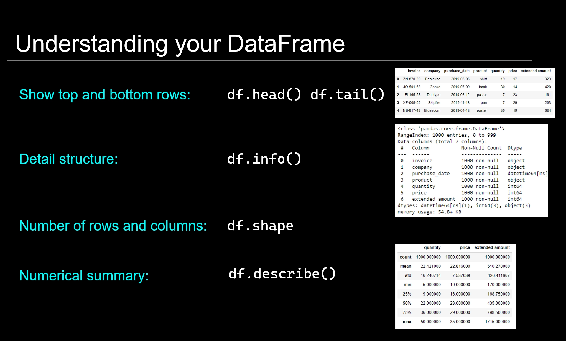
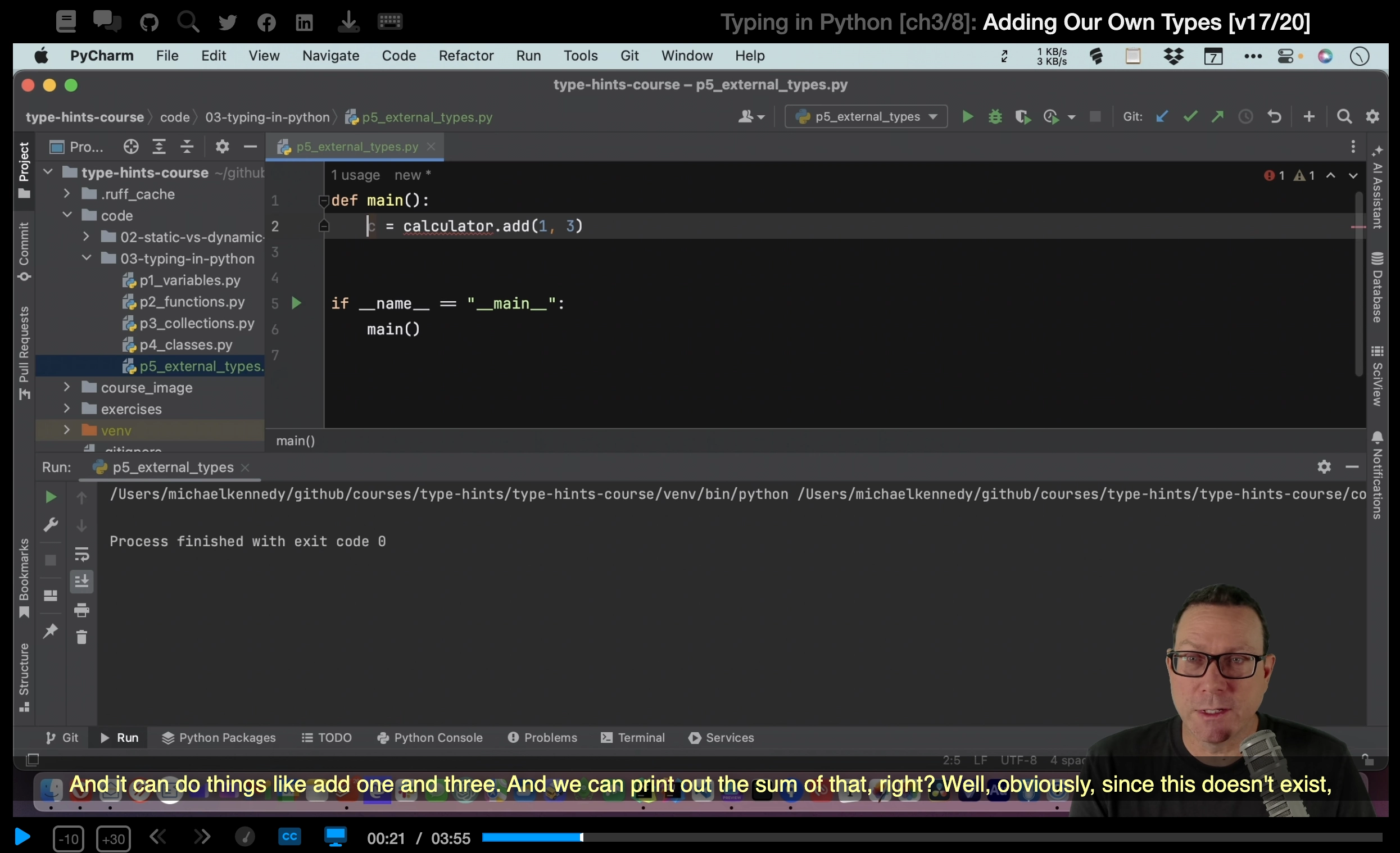
 Hi, I'm Chris Moffitt. I am passionate about finding ways to use the power of Python to be more efficient and effective in a business setting. I've been using Python for over 15 years to solve a variety of real-world problems for everything from web development to system administration and most recently data science.