|
|
|
7:39 |
|
|
show
|
4:02 |
Hello and welcome to RESTful APIs with Eve and Mongo.
This is your host, author and instructor Nicola Iarocci.
I am really excited to share how you can leverage the Eve framework to build and deploy powerful and yet simple REST services in Python.
So let's start with a quick overview of where we're going.
First, we will look at what tools we'll be using during the course and how to store them, maybe you are already confident with some of them or maybe you aren't.
Either way, I suggest you tag along so you get an idea of what is needed for the course and don't have to catch up later on.
Next, we look at REST itself, what REST actually is why it is important and what are some of the core principles that you really want to understand before you even start building a REST service.
We'll also look at few examples of very well known REST services just to get an idea of what is out there and what kind of service we aim to build.
Next up is Flask.
Flask is a simple and elegant micro web framework the Eve framework itself is built top of Flask so making ourselves acquaint with Flask makes a lot of sense.
In this lecture, we will actually build a simple Flask application.
Since Eve shares so many features with Flask our newly acquired skills will come in handy once we move up to the Eve framework itself.
What will follow is an introduction to the Eve framework what features it brings to the table, why and how it allows us to quickly build and deploy powerful RESTful web services and what are its core concepts and philosophies.
Once we are done with this lecture we will have a much clearer idea of what we can do with this technology and why it is so useful to us.
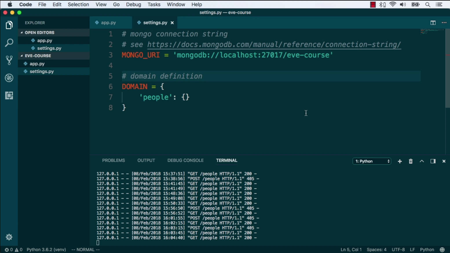
As you probably know already, Mongo is a scalable, high-performance No SQL database.
In my opinion, it makes an excellent choice as a data backend for RESTful services.
In this lecture, we will glance at the feature that makes Mongo a good match for the Eve framework and the reasons why of all possible databases I picked Mongo as the default backend for Eve.
Alright, at this point we will be ready to build our first RESTful services.
In this hands-on section we will make ourselves comfortable with Eve, we will look at the typical application structure, at the set is needed to tailor our app to suit our specific use case.
Finally, we will write some code which will allow us to launch our service.
Since we have a working service now we'll probably want to consume it with a kind of client.
In this section, we will look at how to consume a REST service with Python, Javascript and other tools.
Of course, because REST is not confined to Python or any other specific language or stack, what we will learn here, will be useful to access all kinds of RESTful web services not just our own.
Now that we are capable of sending or receiving data in a RESTful way we want to make sure data coming in is properly validated, this is a wider part of our data service as you can imagine.
In this data focused lecture we will look at how Eve allows to easily set up powerful data validation rules, not only that, we will also see how we can leverage some advanced Eve features to circumvent some of the Mongo limitations, like the lack of joints.
And finally, real-world services.
This is where our Eve service grows up and becomes a mature and fully featured restful service.
We will look at queries and how we can fine tune all kinds of query related features; we will address stuff like pagination, sorting, client server projections, conditional requests, concurrency control, JSON and XML rendering, etc.
We will also get our feet wet with the security management and access control, and of course, production deployment.
|
|
|
show
|
1:02 |
It's time to meet your instructor.
I am Nicola, hey, nice to meet you!
I'm excited that you are taking my class.
I live in Ravena, Italy, where I run a software company that makes accounting apps for small businesses.
I am a Microsoft MVP, a MongoDB Master, a speaker at local and international conferences and a teacher.
In my spare time, I also run the local CoderDojo, a coding club for kids, and DevRomagna, the leading developer community in my area.
What is probably more relevant to you however, is that I am the author and maintener several Python and C# open source projects one of them being the Eve Rest framework.
I have been leading the Eve project and its ecosystem for five years now so as you can imagine, I am quite involved with it and I am looking forward to share my knowledge with you.
If you want to learn more about me and my activity, check out my website that nikolaiarocci.com or follow me on Twitter.
|
|
|
show
|
0:30 |
Of course, I am going to show you a lot of code.
I strongly suggest that you build your own little experimental repo and then try to carefully reproduce and improve on my examples, but do know that everything you see me type is also available on github for you to fork, star or download and play with.
You will find all the course material at talkPython/eve-building-restful-mongodb-backend-apis-course.
So please got here and make sure you star or fork it right away.
|
|
|
show
|
2:05 |
Welcome to your course i want to take just a quick moment to take you on a tour, the video player in all of its features so that you get the most out of this entire course and all the courses you take with us so you'll start your course page of course, and you can see that it graze out and collapses the work they've already done so let's, go to the next video here opens up this separate player and you could see it a standard video player stuff you can pause for play you can actually skip back a few seconds or skip forward a few more you can jump to the next or previous lecture things like that shows you which chapter in which lecture topic you're learning right now and as other cool stuff like take me to the course page, show me the full transcript dialogue for this lecture take me to get home repo where the source code for this course lives and even do full text search and when we have transcripts that's searching every spoken word in the entire video not just titles and description that things like that also some social media stuff up there as well.
For those of you who have a hard time hearing or don't speak english is your first language we have subtitles from the transcripts, so if you turn on subtitles right here, you'll be able to follow along as this words are spoken on the screen.
I know that could be a big help to some of you just cause this is a web app doesn't mean you can't use your keyboard.
You want a pause and play?
Use your space bar to top of that, you want to skip ahead or backwards left arrow, right?
Our next lecture shift left shift, right went to toggle subtitles just hit s and if you wonder what all the hockey star and click this little thing right here, it'll bring up a dialogue with all the hockey options.
Finally, you may be watching this on a tablet or even a phone, hopefully a big phone, but you might be watching this in some sort of touch screen device.
If that's true, you're probably holding with your thumb, so you click right here.
Seek back ten seconds right there to seek ahead thirty and, of course, click in the middle to toggle play or pause now on ios because the way i was works, they don't let you auto start playing videos, so you may have to click right in the middle here.
Start each lecture on iowa's that's a player now go enjoy that core.
|
|
|
|
20:06 |
|
|
show
|
2:08 |
In this module we're going to learn about how to use pandas to read zip files and then we're going to look at the PyArrow data type that is new in pandas 2.
I'll also show you some things that I like to do with data when I get a new dataset.
Let's get started.
Our goal for this project is to understand some student data.
What we're going to do is show how to load it from a zip file, look at some summary statistics, explore correlations, look how to explore categorical columns, and make some visualizations about this data.
|
|
|
show
|
5:26 |
So the data we're going to be looking at is from University of California, Irvine's machine learning repository.
This is a data set of student performance from Portugal.
Let's load our libraries.
I'm loading the pandas library, and I'm also loading some libraries from the Python standard library to help me fetch files from the internet and read zip files.
The data is located at the University of California, Irvine in the zip file.
And if you look inside of the zip file, there are various files inside of it.
We are worried about the student mat csv file.
So what I'm going to do is I'm going to download the zip file using curl.
You'll note in this cell at the front of the cell, I have an exclamation point indicating that I am running an external command.
So curl is not a Python command, but I have curl installed on my Mac machine, and this is using curl to download that data.
Once I've got this zip file, I have it locally.
I can look at it and see that it has the same files.
Now pandas has the ability to read csvs in zip files if there's only one csv in the zip file.
In this case, there are multiple csv files inside of it.
So I'm going to have to use this command here, combine the zip file library with pandas to pull out the file that I want from that.
Let's run that.
It looked like that worked.
I've stored the result df in this df variable.
Let's look at that.
This is a data frame.
We're going to be seeing this a lot in this course.
A data frame represents a table of data.
Down the left-hand side in bold, you see the index.
In this case, it's numeric.
Pandas puts that in for us if we didn't specify one.
There are 395 rows and 33 columns.
So we're only seeing the first five rows and the last five rows.
We're actually only seeing the first 10 columns.
And the last 10 columns, you can see that there's an ellipses in the middle, separating the first 10 columns from the last 10 columns.
And you can also see that there's an ellipses separating the first five rows from the last five rows.
Now, once you have a data frame in pandas, there are various things you can do with it.
One of them might be to look at the memory usage.
I'm going to look at the memory usage from this data frame.
And it looks like it's using 454 kilobytes of memory.
Now, one of the things that pandas 2 introduced is this pyarrow backend.
So I'm going to reload the file using dtype backend as pyarrow and engine is equal to pyarrow.
It looks like that worked.
Let's look at our memory usage now.
And we see that our memory usage has gone to 98 kilobytes.
Prior to pandas 2, pandas would back the data using numpy arrays.
And numpy arrays didn't have a type for storing stream data.
So it was not really optimized for storing stream data.
Pandas 2, if you use pyarrow as a backend, does have a stream type that we can leverage.
And that's probably where we're seeing the memory usage.
Now, we are getting that memory savings by saying dtype backend is pyarrow.
So instead of using numpy, the dtype backend parameter says use pyarrow to store the data.
The other parameter there, engine is equal to pyarrow, is what is used to parse the CSV file.
The pyarrow library is multi-threaded and presumably can parse files faster than the native pandas parse.
Okay, the next thing I want to do is I want to run this microbenchmark here.
And that's going to tell us how long it takes to read this file using pyarrow as the engine.
And it says it takes six milliseconds.
Let's run it without using pyarrow and see how long that takes.
Now, %%timeit is not Python code.
This is Cell Magic.
This is something that's unique to Jupyter that allows us to do a microbenchmark.
Basically, it's going to run the code inside the cell some amount of time and report how long it took.
Interestingly, in this case, it looks like we are not getting a performance benefit from using the pyarrow engine to read the CSV file.
It looks like it's a little bit slower.
When you're running a benchmark with Python, make sure you benchmark it with what you will be using in production, the size of the data that you will be using in production.
In this case, we saw that using that pyarrow engine actually didn't help us.
It ran a little bit slower.
But the number is so small that it's not really a big deal.
If you have minutes and you're going to seconds, that can be a huge savings.
Another thing that you can do with Jupyter is you can put a question mark after a method or a function and you can pull up the documentation here.
You see that read CSV has like 40 different parameters.
If we scroll down a little bit, I think we'll find engine in here.
Let's see if we can find it.
And there it is right here.
So let's scroll down a little bit more.
There is documentation about engine.
So let's read that.
Here it is.
It says that this is the parser engine to use.
The C and pyarrow engines are faster, while the Python engine is currently more feature complete.
The pandas developers have taken it upon themselves to write a CSV parser that will read 99.99% of CSVs in existence.
The pyarrow parser is not quite as feature complete, but can run faster on certain data sets.
To summarize, we've learned that we can use pandas to read CSV files.
We also learned that pandas 2 has some optimizations to make it use less memory.
|
|
|
show
|
3:42 |
In this section, we're going to look at summary statistics for that student data that we just loaded.
Let's get going.
Here's the summary statistics.
This is taken from that University of California, Irvine website.
We've got multiple columns in here describing a student.
And at the bottom here, we've got grades.
This data set was used to look into what features impact how a student performs on their grades.
And we see that there's a G1, G2, and G3, which are the grades.
Now I'm not really going to get into modeling in this section here, but we will look at some of the summary statistics.
So the first thing I generally do when I've got a data set is I'm going to look at the types of the data.
And with Pandas, we can say .dtypes.
This is going to return what's called a Pandas series.
And in the index of this series, we see the columns, and on the right-hand side, we see the types.
In this case, you'll notice that in brackets, we have PyArrow indicating that we are using PyArrow as the back-end, and we have optimized storage there.
We also see that there's int64s.
So those are integer numbers that are backed by PyArrow.
They're using 8 bytes to represent the integer numbers.
And we're not seeing any other types other than strings and integers here.
Another thing I like to do with Pandas is do this describe method.
I was once teaching this describe method to some of my students when I was doing some corporate training, and when I did it, someone went like this and hit themselves in the head, and I asked them, what?
What happened?
Did I say something wrong?
And they said, no, but we just spent the last three weeks implementing this same describe functionality for our SQL database.
So this is one of the nice things about Pandas.
It has a bunch of built-in functionality that makes it really easy.
Describe is one line of code, and you get a lot of output from it.
So this is returning a Pandas data frame.
Pandas is going to reuse a data frame and a series all over the place.
In this case, the index is no longer numeric.
In the bold on the left-hand side, we can see count, mean, std, min.
That's the index.
You can think of those as row labels.
Along the top, we have the column names.
These correspond to the original column names, but these are the numeric columns.
So for each numeric column, we have summary statistics.
Count has a specific meaning in Pandas.
Generally, when you think of count, you think of this as how many rows we have.
In Pandas, count doesn't really mean that.
It means how many rows don't have missing values.
You just need to keep that in mind when you're looking at that count value.
Mean, that's your average.
Standard deviation is an indication of how much your data varies.
We have the minimum value.
At the bottom, we have the maximum value.
In between there, we have the quartiles.
I like to go through this data and look at the minimum values and the maximum values to make sure that those make sense.
Maybe look at the median value, which would be the 50th percentile.
Compare that to the mean to get a sense of how normal or how skewed our data is.
Also, look at those counts to see if we have missing values as well.
In this case, it looks like most of our data is 5 or below.
We do have some going up to 22 or 75, but most of it is not very high.
It doesn't look like we have any negative values.
Now, remember, we just looked at that Dtypes attribute, which said that we are using 8-byte integers to store this information.
Most of these values don't need 8 bytes to store them.
In fact, all of them could be represented with 8 bits of memory.
We could use pandas to convert these integer columns to use 8 bits instead of 8 bytes for each number.
That would use 1 8th the amount of memory.
We could shrink this data even further than we got by using PyArrow without any loss of fidelity in our data.
There are a bunch of other things that we can do.
One of the methods is the quantile method.
I'm going to run that.
This actually failed.
Let's scroll down and look at the error here.
It says, arrow not implemented.
It says, function quantile has no kernel matching input type strings.
The issue here is we have non-numeric columns.
To get around that, we can specify this parameter, numeric only is equal to true.
This is going to give us back a series.
Why did this give us back a series?
Because this is an aggregation method.
You can think of our original data as 2 dimensions.
We are taking the quantile, the 99th percent quantile.
That is taking each of those columns and telling us what's the 99th percentile of that.
It's collapsing it to a single value.
Because we have 2 dimensions, we're going to collapse each of those columns to a single row.
Pandas is going to flip that and represent that as a series where each column goes in the index and the 99th percentile goes into the value.
You'll see that Pandas uses data frames and series all over the place.
You need to get used to these data structures.
The quantile method has various parameters that you can pass into it.
In Jupyter, I can hold down shift and hit tab to pull up that documentation.
You can see that this Q parameter, the first parameter, accepts a float or an array-like or a sequence-like parameter.
In this case, instead of passing in 0.99, a scalar value like I did above, I'm going to pass in a list.
Let's say I want the first percentile, the 30th percentile, the 50th percentile, the 80th percentile, and the 99th.
When we do that, instead of getting back a series, we're now going to get back a Pandas data frame.
But if you look in the index here, the index is the quantiles that we asked for.
This illustrates that power of Pandas that you can do relatively complicated things with very little amount of code.
Also, you need to be aware that this is kind of confusing in that you can call the same method and it might return a one-dimensional object or it might return a two-dimensional object depending on what you're passing into it.
In this section, we looked at summary statistics of our data.
Once you've loaded your data into a data frame, you're going to want to summarize it to understand what's going on there.
That describe method is very useful.
Then there are various other aggregation summaries that we can do as well.
as well.
I showed one of those which is
|
|
|
show
|
2:28 |
I want to explore correlations.
Correlations are the relationships between two numeric columns.
And this is a good way to understand if one value is going up, does the other value go up or down or does it have no impact on it.
So let's see how we can do that with pandas.
I'm going to say df.core and I'm going to pass in that numeric only because otherwise it's going to complain about that.
And look at what this returns.
It's a data frame.
In the index we have all the numeric columns and in the columns we have all the numeric columns.
In the values here we have what's called the Pearson correlation coefficient.
This is a number between negative one and one.
A value of one means that as one value goes up the other value goes up in a linear fashion.
If you were to scatter plot that you would see a line going up and to the right.
A correlation of negative one means that if you scatter plotted it you'd see a line going down and to the right.
A correlation of zero means that as one value is going up the other value might go up or down.
You might see a flat line but you also might see alternating values.
As one value increases the other value may or may not increase.
They don't have a relationship to each other.
Now humans are optimized for looking at big tables of data like this.
Generally what I want to do when I have this correlation table is to look for the highest values and the lowest values.
But I might want to look for values around zero and it's kind of hard to pick those out.
If you look you might notice that along the diagonal we do see a bunch of ones and that's because the correlation of a column with itself is the column goes up the column goes up.
So you do see that value there but we're actually not interested in that value.
We want to look at the off diagonal values.
So let me give you some hints on how we can do this.
One of the things that pandas allows us to do is add a style.
So I'm going to use this style attribute and off of that I can say background gradient.
Let me note one more thing here.
This is showing how to use what's called chaining in pandas.
I'm actually doing multiple operations to the same data frame here and I put parentheses around it.
What that allows me to do is put each step on its own line and that makes it read like a recipe.
I'm first going to do this then I'm going to do this then I'm going to do this.
Do I need parentheses?
No I don't.
If I didn't use parentheses I would have to put all of that code on one line and it gets really hard to read.
So I recommend that when you write your change you put parentheses at the front and then parentheses at the end and then just space it each operation on its own line.
It's going to make your life a lot easier.
Okay so what we've done is we've added this background gradient.
The default gradient here is a blue gradient.
It goes from white to blue, dark blue.
Again along that diagonal you do see the dark blue but this is actually not a good gradient.
What we want to use when we're doing a heat map of a correlation is to use a color map that is diverging.
Meaning it goes from one color and then hopefully passes through like a light or white color and goes to another color.
That way we can look for one color for the negative values and the other color for the positive values.
So let's see if we can do that.
I'm going to specify a diverging color map.
That's the RDBU, the red blue color map.
And it looks like we are seeing those diverging values now.
Now there is one issue with this.
The issue is that if you look for the reddest values I'm seeing pretty red values for example around negative 0.23.
That's not negative one and I would like my red values to actually be at negative one because I also want my white values to be around zero.
If I look at my white values it looks like they're around 0.42 right now.
Note that the blue values are at one.
Again that's because that diagonal by definition is going to be one.
So pandas has an option for us to do that.
We can specify these Vmin and Vmax values to specify where those get pinned down.
And when we do that we actually get a proper coloring here.
Now this makes it really easy to find the reddest values and I can see that failures have a large negative correlation with the grade.
Again we do have that diagonal there but we want to look at the off diagonal values for correlations.
And over there at grades we can see that grades are pretty highly correlated with each other.
Probably makes sense that if you did good on the first test you probably did good on the second test etc.
Another thing that you can do with the correlation is you can change the method.
I can say instead of doing the Pearson correlation coefficient which is the default one I can do a Spearman correlation.
A Spearman correlation does not assume a linear relationship rather it's also called a rank correlation.
So you might see if a relationship if you did a scatterplot it curves like that.
That could have a correlation of one as the rank of one goes up the rank of the other one goes up but it's not a linear correlation.
So oftentimes I do like to do a Spearman correlation instead of the Pearson correlation which is the default value.
In this section I showed you how to look at correlations.
I showed you one of my pet peeves I often see in social media and other places people showing these correlation heatmaps and they'll throw a color on them but they don't pin those values.
So make sure you use a diverging color map when you're coloring this and make sure you pin those values so that the negative value is pinned at negative one and that light value goes at zero.
|
|
|
show
|
0:48 |
In this section, I'm going to take you through what I like to do with categorical columns.
So let's get going.
First of all, let's just select what our categorical columns are.
In Pandas 1, we would do it this way.
We would say, select D types object.
Again, that's because Pandas 1 didn't have a native way to represent strings, and so it used Python strings, which are objects in NumPy parlance.
In Pandas 2, we do have that ability.
So if we do say string here, we get back a data frame and all of the columns here are string columns.
Now, I want to summarize these.
I can't use those same summary statistics that I did use with describe up above, but I can do some other things and I'll show you those.
Alternatively, we could say select D type string and then square bracket, pie arrow, that gives us the same result in this case.
Is there any value to that?
Not necessarily.
It's a little bit more typing.
I want to show you my go-to method.
So when we're doing a lot of these operations, I like to think as Pandas as a tool belt.
It has 400 different attributes that you can do on a data frame and 400 different things that you can do to a series.
Do you have to memorize all of those?
No, you don't.
But I want to show you common ones and you can think of them as tools.
You put them in your tool belt and then we use these chains to build up these operations.
Your go-to when you're dealing with string or categorical data is going to be the value counts method.
Let's look at that.
Let's assume that I want to look at this fam size, which is the size of the family.
You can see the column over here, but let's explore that a little bit more.
So all I'm going to do is I'm going to say, let's take my data frame, pull off that fam size column, and then do a value counts on that.
What this returns is a Pandas series.
Now, let me just explain what's being output here because it might be a little bit confusing.
At the top, we see fam size, and that is the name of the column or the name of the series in this case.
Then on the left-hand side, we see GT3 and LE3.
Those are the values and they are in the index.
The actual values of the series 281 and 114 are on the right-hand side.
At the bottom, we see name.
Name is count.
So that is derived from doing value counts there.
We see D types.
It says this is an int64.
So the type of the series is a PyArrow int64.
Let's do the same thing for higher.
We'll do value counts, and you can see that we get back a series with those counts in that.
Now, if we want to compare two categorical or string columns with each other, Pandas has a built-in function to do that called cross tab or cross tabulation.
What that is going to give us is a data frame, and we'll see in this case we have sex in the index and higher in the columns, and then it gives us the count of each of those.
This has various options.
Again, we can put our cursor there, hold down shift and hit tab four times there to pull up the documentation.
So there's a lot of things we can do.
Turns out Pandas has pretty good documentation.
So check that out if you want to.
I'm not going to go over all that right now.
But an example is we can say normalize.
Now, instead of having the counts there, we have the percentages, and this is normalized over all of the values in there.
If I want to format that and convert that into a percent, we can say style.format, and now I'm getting percents there.
I can say I want to normalize this across the index.
So what does that do?
It says I want to take each row and normalize each row.
So we're going down the index and normalizing each row.
I think that normalizing across the index is a little bit weird.
To me, this seems backwards.
To me, it seems like we're normalizing across the columns instead of the index.
But if we want to normalize down a column, then we would say normalize columns there, and we're normalizing down the columns that way.
Pandas has some warts.
I'll be the first to admit it.
And oftentimes, when we are doing aggregation operations, if we want to sum across the columns, we would say axis is equal to columns, and we would sum across the columns.
In this case, this normalize here seems a little bit backwards, but we'll just deal with it.
It is what it is.
In this section, I showed you how I would look at string data.
Generally, I'm going to take that value counts and quantify what is in there.
Oftentimes, we can see whether we have low cardinality, if we have few unique values, or if we have all unique values, we can see that relatively quickly.
If I want to compare two categorical values, I'm going to use that cross tabulation to do that.
|
|
|
show
|
4:48 |
In this section I want to show you some visualizations that you can do really easily with pandas.
So if I've got a numeric column, I like to do a histogram on it.
So I'm going to say, let's take the health column, which is this numeric value from 1 to 5.
And this is the health of the student.
And all I do is say pull off the column and then say .his.
Now I am saying fig size is equal to 8,3.
Fig size is a matplotlib-ism.
This is leveraging matplotlib.
Now you do see a space in here around 2.5.
The issue here is that by default we are using 10 bins here and these values only go up to 5.
So I might want to come in here and say bins is equal to 5 and change that.
Oftentimes people say they want to look at a table of data.
And again, humans aren't really optimized for that.
If I gave you a table of the health column and said like, what does this have in it?
It's hard for you to really understand that too much.
But if you plot it, if you visualize it using a histogram, it makes sense.
And that's a great way to understand what's going on with your data.
Let's just take another numeric column.
We'll take the final grade and do a histogram of that.
In this case, I'm going to say bins is equal to 20 because this value goes up to 20.
This is really interesting to me.
You can see that there's a peak there at 0, indicating that you do have a large percent of people who fail.
And then it looks like around 10, you have another peak.
That's probably your average student.
So this is illustrating not a bell curve, so to speak, but the distribution of grades, which I think is interesting.
And it tells a story just by looking at this.
Again, could we tell this by looking at the column of data?
It would be really hard to do.
But giving that plot there makes it relatively easy.
If I have two numeric columns and I want to compare them, I like to use a scatter plot.
We're going to plot one value in the x-axis and another value in the y-axis.
Pandas makes it really easy to do this as well.
What we're going to do is we're going to say df and then an attribute on the data frame is plot.
And from that plot, we can do various plots here.
So one of those is scatter.
In fact, there's also a hist there as well.
So hist is on data frame and it's on a series directly.
But also those are both available from the plot accessor.
In order to use the scatter plot, we need to say what column we want to plot in the x-direction and what column we want to plot in the y-direction.
So we're going to plot the mother's education in the x-direction and their final grade in the y-direction.
And I'm just going to change the size of that so it's 8 by 3.
Here's our plot.
When I look at this plot, a couple of things stand out to me immediately.
One is we see these columns.
One is that we see values at regular intervals here.
So this tells me that we have gradations that are at some level, which kind of makes sense.
Our grade is at the whole number level.
You don't have like a 15.2 or a 15.1.
You just have 15, 16, 17, et cetera.
Makes it very clear when you see the scatter plot.
The other one is that we're seeing columns there.
And so you can think of the mother's education, it is a numeric value, but it's also somewhat categorical in that it's lined up in columns.
So I'm going to show you some tricks to tease that apart and understand what's going on here.
If you just look at this plot on its own, it's hard to tell where the majority of the data is.
So I'm going to show you how we can find out what's going on behind this plot.
One of my favorite tricks with a scatter plot is to adjust the alpha.
Now, if I just see a bunch of dark values there, what I want to do is I want to lower that alpha, which is the transparency, until I start to see some separation there.
I think that looks pretty good.
I might even go a little bit lower.
You can see that I'm now starting to see some faded values here.
So by looking at this, this tells a different story to me than this value up here.
This is telling me that we have more values at 4.
How do I know that we have more values at 4?
Because it's darker there when we lowered the alpha.
We're not really seeing that so much on this plot.
What's another thing we can do?
Another thing that we can do is add jitter.
Basically, we'll add a random amount to the data to spread it apart and let us see what's going on inside of that.
So I'm going to add jitter in the x direction to spread apart that mother's education value.
I'm going to use NumPy to do that, and this is going to use the assign method.
The assign method lets us create or update columns on our data frame.
I'm going to say let's make a new column called EduJit, and it's going to consist of the mother's education plus some random amount.
I'm using NumPy random to generate some random values there.
In this case, the amount is 0.5.
I don't want my random values to overlap values from another value, so I'm keeping them within a certain width.
Then I'm going to say on that new data frame, let's plot that.
Let me just show you that this is pretty easy to debug once you have these chains here.
You can actually say here's my data frame, and then I want to make a new column.
There is my new column.
It popped over there on the end.
Now once I have that, I'm going to plot the new column in the X direction and plot the grade in the Y direction.
We get something that looks like this.
This also tells us a different story than this one up here.
I think this is a much better plot, letting us see where the majority of the data is.
Now I have inlined that Jitter functionality right here, but it's pretty easy to make a function to do that.
I'm going to write a function down here in this next one called Jitter.
Then to leverage that, I'm going to say, okay, EduJit is now this result over here.
Now let's explain what's going on here.
On the right-hand side of a parameter in a sine, up above here you can see that we passed in this is a series, and we're adding some amount to it.
This is a Pandas series up here.
Down here, this is a lambda function.
We can pass in a lambda function on the right-hand side.
What happens when we pass in a lambda function?
When you have a lambda function inside of a sine, Pandas is going to pass in the current state of the data frame as the first parameter to that lambda function.
Generally, you will want that lambda function to return a series because you want that to be what the column is.
Now do you have to use lambdas?
No, you don't have to use lambdas.
You can use normal functions as well.
Oftentimes, it is nice to use lambdas because you want that logic directly there inside.
When you're looking at your code, the logic's right there.
If you were to repeatedly use the same lambda all over the place, then I might recommend moving that out to a function so you only have to write it one place.
Let's run that and make sure that that works.
That looks like that works as well.
If this jitter was useful, what I would do is make a helpers file, and I would stick that jitter into the helpers file so I can leverage that.
I also want to look at how to visualize string data.
What I'm going to do is I'm just going to tack on a plot.bar into my values count.
When we do a bar plot in Pandas, what it does is it takes the index and it puts it in the x-axis.
Then each of those values for those index values, it plots those as bar plots.
Once you understand that, it makes it really easy to do bar plots.
Let's see what happens when we run .plot.bar.
We should see mother and father and other go into the x-axis.
We do see that.
This is a little bit hard to read because I have to tweak my head to the side.
Generally, when I'm making these bar plots, I prefer them to be horizontal.
To make a horizontal bar plot, I just say bar h.
There we go.
There's our visualization of that.
We can see that most of the guardians are actually the mother in this case.
In this section, we looked at how to visualize your data.
I'm a huge fan of visualization because I think it tells stories that you wouldn't get otherwise.
Once you understand how to make these visualizations in Pandas, it's going to make your life really easy.
|
|
|
show
|
0:46 |
Okay, I hope you enjoyed this module.
We looked at loading some data and doing some basic exploratory data analysis, trying to understand what's going on with our data.
These are steps, tools that I will use every time that I load data.
So I want you to make sure that you understand these, but you start practicing them as well because they'll apply to most data sets that are in tabular form.
|
|
|
|
7:11 |
|
|
show
|
7:11 |
So what is Rest all about?
At conferences or even while talking to my colleagues I am often surprised by how much confusion there is even to these days about what really Rest is.
In this section we're going to talk a little bit about Rest and RestFul web services just to make sure that we understand what kind of service we're going to build with Flask and Eve.
The first thing you need to understand and embrace is the surprising fact that Rest is not a standard and also, it is not a protocol.
Rest is more really an architectural style for networked applications.
Now, architectural style may sound cool and probably is because by not imposing hard to use, it allows for great flexibility.
On the other hand, quite frankly, it sucks.
Probably, on the internet, there aren't two APIs who share the same interface or behavior, most of them however have tier in some way or another to Rest principles.
So let's review a few of these important principles.
First, and probably the most important is the resource or the source of a specific information.
By the way, in Rest terms, a web page is not a resource it is rather the representation of a resource.
If you access your Twitter timeline for example what you are seeing there is a representation of the thoughts expressed by the people you are following; second important principle is the global permanent identifier, global being key.
URLs allow us to access the very same resource representation from any place in the world which is not a small feature if you think about it.
Third, standard interface.
Rest was defined in the context of http and in fact, https are very common standard interface but very few people know that Rest could actually be applied to other application layer protocols.
There is also a number of constraints that RestFul web services are supposed to be following stuff like separation of concerns, stateless, cacheability, being layered systems etc.
We will get back to these in a few minutes.
So in a way we could say that the worldwide web is built on top of Rest and it is meant to be consumed by humans while RestFul web services are also built on Rest and are meant to be consumed by machines.
So let's review these Rest principles.
The most important thing is that we're communicating over http we have a service, it's using http or https and it's explicitly using all the concepts and mechanisms built into the http itself.
So status code, verbs such as get, post, put, delete, content types, both for the inbound data and the outbound data.
There are many services out there that have been built technically on http as transport layer but they ignore all of these things and they aren't RestFul services at all.
Next, the endpoints that we took into our URLs and this typically means that when we design our service we're thinking in terms of nouns.
So maybe I'm designing a bookstore and I might have a books or works endpoint I wouldn't have a get books or add books or even books-add, no, you just have one single books endpoint and you apply the http verbs to modify them.
Do you want to get all the books?
We'll do a get request against books endpoint.
Do you want to load the new one let's do a post request to that endpoint.
So you combine these http concepts, codes and verbs and you apply them to these endpoints so really, the take away here is when you design these APIs you need to think in terms of nouns and what are the things being acted upon your system.
Responses for your request should also be cacheable if the responses are cacheable you get a huge performance boost like in a get request against the books endpoint it might be served by an intermediate proxy server that cached the same response beforehand.
We also want to make sure that our system is a layered one and what that means is that our service clients cannot see past our API surface.
If our service is calling through other services and it's composing them to basically make up its own functionality, that should be opaque to our consumers.
Our services should also be stateless we should be able to make requests, data response, and that's all we need to know.
We don't log into the service and then do a batch of operations and then log out.
If you have to carry that authentication maybe we have to pass some kind of token as a header value or something like that.
RestFul service should have support for content negotiation so let's take our book example, the books-1 endpoint might give us book one.
Well, how do you want that?
Do you want that in xml, do you want that in Json, do you want maybe the picture that is the cover page?
We could have a bunch of different endpoints but typically, these RestFul services will support content negotiation, so if we make a request to that url and we specify that we want Json, well we should get the Json representation of the book back, but if we specify one image png then maybe I should get back the cover picture for that book.
So that's content negotiation.
Finally, we have a thing called HATEOAS or hyper media as the engine of application state.
Now this is less used, but some RestFul services do make use of HATEOAS and the idea is that I make a request to the service and in that response, maybe I have other URLs relative to the current endpoint, in my interaction with it, maybe I can follow those URLs further, so I go like, hay bookstore what do you got and it says well, I have books and I have authors and if I follow authors, maybe it says well, here is a bunch of people that you can go look at etc.
Just think of a HATEAOS as a way for clients to explore and navigate the RestFul service by following its links.
Alright, we've seen a number of constraints and features that RestFul services are supposed to be providing to clients.
There are a lot of them as we've seen, some are more complex than others, but the good news is that when you build a service on top of Eve, all of these features and constraints are supported and already provided for you.
You can, of course, switch some of them on and off, but in general, Rest assured that the web service you're going to build on top of Eve is going to be a fully featured RestFul web service.
|
|
|
|
11:43 |
|
|
show
|
4:13 |
Before we dwell on Eve itself, we really need to talk about Flask.
Why, you ask?
Firstly, because Eve is built on top of Flask, keep that in mind because it is very important and powerful.
Anything you can do with Flask, you can also do with Eve, that is remarkable, because by leveraging Flask and Eve, you end up being able to fine tune, extend and customize basically every single feature that comes with the framework itself.
So in this section, we will make ourselves comfortable with Flask and trust me, it will be worth it.
Once we move on to Eve in the next sections you will be amazed at how comfortable you feel sitting at the Eve wheel.
Now if you look at the Flask about page you see that Flask tags itself as a micro web development framework, what does it really mean?
Micro doesn't mean that the web app has to fit into a single Python file of course, nor does it mean that Flask is lacking in functionality.
The micro in micro framework actually means that Flask aims to keep the course simple, but extensible.
Flask want to make many decisions for you such as what database to use, those decisions that it does make however, are easy to change.
Everything else is up to you so that Flask can be everything you need and nothing you don't.
Again, being micro doesn't mean lack of functionality, let's look at its acclaimed Restful request dispatching for example; here we are looking at two possible roads for our apo, one, obviously being the home page and the other one being a Hello URL.
As you can see, we are using a decorator to instruct Flask on which functions should be run when a user hits a certain URL or endpoint.
How nice is that?
There is more to it, of course, like the option to add variable parts to you URL to use.
But you can already see how Eve could easily leverage and build on top of this feature to provide an out of the box, yet powerful and easy to use routing mechanism.
Flask also comes with a built in development server and debug support.
This is super important when you are prototyping and then writing web apps.
You get all sorts of debugging formations, like stack traces and variable inspection just by setting an environment variable as we see here.
In the following line, we see how easy it is to launch the application itself.
This is possible, because Flask comes with its own development server which is more than good enough to play and test the app before going into production.
There are many other nice things that are coming with Flask and one of my favorites has got to be the integrated support for unit testing.
When you're building a framework you want to make sure that it is well tested.
That is true for any kind of web app really, but if your end users are going to be developers, well, you want to make your test as complete and effective as possible.
Flask native support for unit testing which we can see at work in this course snippet, is a key feature, and we have of course been abusing it while developing the Eve framework.
If you're going to write your own web apps or frameworks with Flask, you really want to get to know everything about testing Flask and of course, its debug mode and development server.
So Flask is cool and it is fun.
It is easy to set up and use, but being micro by desine doesn't come with the tons of a high level features such as database access or an admin backend.
Luckily and precisely because it is micro, powerful and easy to extend over time a huge number of Flask extensions have surfaced and are now available for you to use.
The extensions' registry is loaded with all kind of useful tools which you can plug into your app and most of the times Eve too, and then be on your way, or you can build your own extension and then contribute it to the community.
In fact, one of the reasons why Flask is so popular is because it is very easy to build on top of it, and in any case, the extension registry is at your fingertips where you don't feel like reinventing the wheel.
|
|
|
show
|
7:30 |
Let's build our first Flask application.
First of all, we want to activate our virtual environment, so let's just source our activation script and here we go, as you can see the virtual environment is now active and we are sitting in our working folder.
We can now launch our text editor we already have a hello.py script in here.
The first thing I want you to note is that we are dealing with just 6 lines of code, actually 4, if we don't factor in the import line here and the blank line, so we are speaking about 4 lines of code for a fully functional Flask app.
I guess this is where the famous, simple and elegant Flask definition comes from.
Let's review our code line by line.
On the first line, we are importing a Flask class from the Flask package.
This class will be our wsgi application.
On the second line, we are creating an instance of our class and as you can see, we are passing an argument.
This is the name of the application module or package and it is needed so Flask knows where to look for templates, static files and so on.
On line 4, we are using the route decorator to tell Flask what URL should trigger our function.
So any time the home page is hit by the browser the hello function will be triggered and the function itself is super simple, it is simply returning a hello world message.
So now our script is ready and we want to see it running, right?
So how do we do that?
We could go back to our terminal window and launch the built in Flask server, but we can do better than that because within code we have an integrated terminal window and we can use it let's just go to the view menu and click on integrated terminal, and here we go, we have a new window with the terminal.
And as you can see, we are already in our working folder and in fact, if we check the contents, we see our hello.py script right there.
Now, before we can continue, we need to activate the virtual environment, so let's do that.
Now we're ready, and by the way, by the time you see this screencast, you probably want to activate the virtual environment yet again because as you might remember, we already activated it before launching the editor.
There is a ticket open on the github repository for Visual Studio Code and a fix to go online with the next update in February 2018.
So now that the virtual environment is ready we can try and launch our script.
To launch the built in server, all we need to do is issue this command Flask run, and if we do that, it will fail, and the reason is that we didn't tell Flask which is the launch script, we can do that by simply exporting the Flask app variable and we set it to our scrap Okay, let's try again, Flask run, there we go, as you can see, now Flask is serving the app hello on local host port 5000.
Let's go and try it out.
Hello world, this is nice, we have a working website up and running with just six lines of Python code and the built in Flask server is serving it to us.
How can we improve it?
Well, first we might want Json as a response since we are going to build RESTful APIs anyway, so how do we do that?
Let's go back to our app, it turns out that Flask comes with a very powerful jsonify function so we can leverage it, and in our function we simply go and call jsonify and then we need to pass a Python dictionary, so maybe something like this, it should be good enough, let's save, go back to our browser and refresh.
And nothing happens.
Why is that?
Well, the reason is that we didn't relaunch our server so let's stop the server and launch it again, so it can pick the new script, and here we go, as you can see, now we're getting Json back as a response to our request.
Now, powerful, but it is quite annoying that we have to stop the server and relaunch every single time we make a change in our scripts.
Well, luckily for us, Flask comes with a built in debug mode, and we can activate it by simply setting an environment variable, so let's do that.
Again, let's stop the server and export Flask debug let's switch this variable on.
And now, let's run the server again.
As you can see, we get a slightly different message now the Flask app is running but it is forced to debug mode, so now, any change we do here, it will be picked up by the server.
Let's try for example and add a new route— how about we make a log in page, okay, let's save, and we can see that the server here has detected a change in hello.py and it is reloading, in fact, the server restarted and let's see if we go back and just go to the login page there it is, we didn't need to stop the server, so for example, let's say that we change the contents of the string in welcome, you are logged in, save, again, the server restarts, we go back, refresh, here we go, back to our script, we only scratched the Flask surface here, of course, there is a lot more to Flask to be seen but I believe in a few minutes, we achieved quite a lot we now have our Flask site up and running, we know how to handle growth with Flask and we also learned how to import some very nice functionality from Flask.
Of course, we learned about the built in server and the debug mode.
All these features will come in handy in the next segments, when we move on to Eve.
|
|
|
|
14:38 |
|
|
show
|
2:06 |
A few years ago, I was assigned to a new, exciting and challenging project— build a fully featured RESTful service for my company.
So, I first researched the REST principles and their concrete implementations.
then, I went on to pick a very db backend for my service.
Right from the beginning, the plan was that soon enough, more REST services will go online to complement the first one, and since I didn't want to reinvent the wheel every single time, I thought it would be smart to build something that would be easily redeployable.
Ideally, I would simple launch a new instance with my package which would, of course, provide all the needed features from the get go.
Then, plug a new data set, set up appropriate validation, authentication and authorization rules, and bam, a new REST API will be online, ready to be consumed by our hungry clients.
If I could provide most of the features with a single, reusable package, and if I could make it so that duties like plugging at different source, extending, customizing the common feature set, well, if all of these would be easy enough, then I would be a winner.
Soon, I realized that such a tool would end up being more a framework than a simple package.
And, more excitingly, it could be useful to a lot of people out there.
The result of that work was presented at the EuroPython conference back in 2012.
My talk there ended up being more of a workshop on how to use Flask and Mongo to build REST services.
But, what I was really looking for was some kind of validation for my project and idea.
That is when basically Eve as an open source framework was born.
So here it is, if you have data store somewhere and you need to expose it through some kind of RESTful services, then Eve is the tool that allows you to do so.
And because it is built on top of Flask, it is very easy to use, as you can see in this snippet here, and also it's easily customizable and extendable.
|
|
|
show
|
6:20 |
If you go to the Eve homepage, at Python-eve.org, you'll find that there's a live demo available for you to play and experiment with.
The source code for this demo is on github, so any time you can go and check it out.
I suggest you do that once we've done with this course you can use this basic app as a reference or a starting point to build your first experimental or advanced REST service.
Thousands of people have been playing and experimenting with it to better assess Eve features and functionalities.
Let's do the same so we can get a gentle introduction to the framework and make ourselves a solid idea of what's coming with the rest of the course.
Now, depending on the browser you are using when you click on this link at the Eve homepage you will get a different result.
I remember getting some xml back from Chrome for example, here I am on Safari and if I click on this link what I get back is basically what appears to be just random strings.
They are not really random, actually the API is working well it's providing us with a nice response and if we look at the address bar, we already get some nice information we are hitting a secured service, this service is hosted on Heroku and if I click on that, I can see that I'm actually hitting the people endpoint.
Now, if we want to better assess what's going on and understand what the response is we really need to switch it to a better client browsers are not really the best option when you want to use and consume our RESTful service.
What we really need is a REST client and as you might remember, we already installed Postman in a previous section of this course, so let's just launch it, and here it is so on Postman we have two panes, on the left side we have the request pane and on the right side we have the response pane, we enter the URL here, let's just pass the same URL we hit before with the browser and click the send button.
After a few seconds, we get response back and as you can see, this is actually readable and if we check on the headers tab here we see that the content type is application Json and that the server is actually an Eve instance.
Now, this service only exposes 2 endpoints one is people the other one is works, here it is.
Now, for both requests we got an OK status back because the endpoints were existing what if we type an endpoint which doesn't exist?
Well, of course, as you might expect we get a not found back from the framework and if we look at the response body, we see that actually some Json is provided back it has two nodes, error which has details about the error, so the error code and the message, which is a human readable explanation of the problem, and a status.
So every time there is an error with a request you get a proper status and also a human readable parsable Json back from the framework, let's go back to our people endpoint now.
Of course, you can define as many endpoints as you want on your service but what if your client can't process Json and needs xml instead.
Well, that's easy because it supports both formats, all you have to do is perform a slightly different request let's go here to the headers tab and say that this time we only accept xml and hit send, as you can see now, we're getting xml, if we go to the response headers tab, we see that actually we are provided with xml.
Let's try again, and switch back to Json, here it is.
Do know that you can configure your service and decide which formats are supported and which aren't.
By default, your service will support both Json and xml but we will see in the following segments that we can switch one of them on and off as we please.
Let's consider the Json response for a moment.
There are 3 main notes, links, items and meta.
Meta is easy, we get the total number of documents matching the query, the page we run and the maximum number of documents we get for every page.
These settings are of course configurable as well as weather pagination is supported or not.
Link has some navigational information for the client and items is an array where we get the actual documents, we already know that we should have seven documents in this array 1, 2, 3, 4, 5, 6, 7, let's pick one, like this one, again, every single document has a links node, with navigational information.
And then, there are some meta fields and you can tell these are meta fields because they are preceded by these underscore here, so here are the unique id for the document, the last time it was updated and etag which is basically a hash of the document and the date the document was created the first time.
The rest are actual document fields like last name, first name, location which, as you can tell, is a subdocument; a role is an array so here we have Mark Green living in New York, and he is both an author and a copy, and he was born on February, 1985.
Now we are looking at the default response, but many features can be disabled for example, if you don't like providing the clients with the links, know that you can disable them, what you can't avoid are the document meta fields like id, updated, etag and created, these are needed by the API you don't need to mess with them, the API will handle them for you and for the clients.
And they are important because they allow the client to perform conditional queries and the server can perform optimized queries on the database.
|
|
|
show
|
2:30 |
Speaking about queries, let's see how we could perform queries against our remote API.
Let's say that we want to find all the people where last name is Green.
So we go over here to the URL and we set a query string we use the where keyword and then we go with a Mongo syntax, you can see here it is basically a Json object so find all the documents where last name is Green.
Let's try this one, and as you can see, we only have one document back and it is exactly what we were looking for, let's try something more complex and find all the documents where last name is Green and also location.city is Ravena, which is my hometown in Italy.
Zero documents back, and that makes sense, it is what we expected, as you can see, the items array is empty.
Now if we go back to my query and replace Ravena with New York I should get back my Green guy again.
Because location city is in fact New York, so as you can see, you can also query on subdocuments, like we did here using the .
syntax you can chain multiple conditions and you can basically use all of the MongoDB supported operators like or, and, etc.
You have also another option, if you don't like the Mongo syntax, maybe you are not familiar with it, you can actually use the Python syntax, which is different, let's try one example where last name=green same result, as you can see.
So different syntax, similar result.
Now we will see in the following segments that you can actually configure your API and decide which syntax you want to support, by default, both of them are allowed, but you can actually turn Python syntax off or Mongo syntax on and off, however you please.
|
|
|
show
|
2:43 |
And what about sorting?
Of course you can sort too, you just have to use the sort keyword in your query definition, so for example, here we are sorting by location.city and then by last name, and because I am using a dash before the last name, field I want then reversed.
So basically I am looking for all the people with no filter, because I am not using the sorted by location.city and last name reversed.
Let's see what happens, we have 7 documents, the first document here has no location subdocument as you can see the second is the same, no location, the third one is in Ashfield and then we have another person living in Auburne, and then New York comes, and then San Francisco, San Francisco again and if we check it on the last names, we will see that they are sorted by diverse order.
For example, we have 2 people living in San Francisco let's go and see, we have miss Julia Red first and then comes Miss Serena Love, so yes, we are getting them in reverse order, of course, we can also mix a filter with sorting, so here we might go with something like where— okay, so here we are looking for all the people living in San Francisco sorted by last name reversed.
Only 2 documents, and we can see they both live in San Francisco and the first one has last name Red and then Love, again, if I remove the dash here I am sorting by last name and we should get the same two documents but the first one is Love this time and the second is Red.
Also, when using sort you might want to switch to a Mongo syntax something like this, which isn't probably very intuitive, but you can do that if you want to, same result, of course.
|
|
|
show
|
0:59 |
And what about pagination?
Well, at this point, you probably have an idea of what you can do, you can use the page keyword here and ask for page 2 for example, so all the people, second page.
Of course, since we only have 7 documents total, and we don't have any document on page 2 because we have 25 documents per page, so they are all going to be on page 1, if we go to page 3, same result, if we go on page 1, we get all of them.
Again, pagination can be disabled, we will see how, it will also improve performance, if you turn it off, but we will talk about that in one of the next segments.
Alright, our tour is over, hopefully you got a general idea of what you can achieve with an Eve powered API.
There are of course many more basic and advanced features and we will learn more about them in the next segments when we start building our very own service.
|
|
|
|
4:28 |
|
|
show
|
4:28 |
In this lecture, we are not going too deep into what Mongo is and how it all works.
You can find all sorts of information about it on the internet.
There is also a Mongo installation lecture in the appendix should you need details on how to properly set it up on your machines.
You might be wondering though why Mongo was picked as the default db engine for the Eve framework, when there were in fact so many other options around, especially in the SQL ecosystem.
After all, when the Eve project was started, Mongo certainly wasn't as popular as it is today.
In fact, the No SQL world have just surfaced on the public scene back then.
In hindsight, I believe it proved to be a great choice, but allow me a few minutes to explain why I thought right from the beginning that Mongo was going to be a perfect match for a RESTful service.
Mongo stores data in flexible Json like documents, meaning, fields can vary from document to document and data structure can easily be changed over time.
But more importantly, as you know, RESTful services usually communicate with the clients via Json.
So let's look at a typical get request, we have a client somewhere and it is accepting the Json media type.
On the other side, we have Mongo, which is storing native Json documents as well.
So maybe we can push directly to the clients from Mongo?
Ideally, yes, there is little working wall as Python dictionaries naturally map to Json documents.
The same holds true when clients are writing to the service.
Here is a post request, Json coming from the client that is received from the service validated and then stored on the database.
And what about queries?
Well, it turns out that in Mongo queries are also represented as Json style documents.
Here we are looking at a query performing in the Mongo shell, now, if you were in SQL world, this will be a typical select all documents from table things where x=3 and y=4.
As you can see, the actual query is in fact a Json document itself.
A Json document is the perfect candidate for a URL query definition, isn't it?
We still need to perform some validation, then, we can simply forward a query to the database.
The result will be of course a Json document again.
So as you can see, we're essentially going to have Json all along the pipeline, or, if you will, Mongo and the REST service are speaking the same language and in general, mapping to and from the database feels more natural.
There is no need to involve any kind of ORMs which would end up making the service more complex and more importantly for us, will probably have an impact on performance.
As we mentioned already, Mongo is schemaless.
Now, this doesn't really mean that we don't need a schema.
most likely, we still want to validate what is coming into our system so we want to define some validation rules for known fields we will see that Eve actually also supports storing of unknown fields and documents.
But that is an opt in.
By default, when you are storing data on your service you're guaranteed that unknown fields are rejected, still, not having to worry about updating your db schema as your service and requirements evolve is very powerful and allows for less downtime not to mention migration headache.
Lastly, let's talk about transactions.
One complaint that you usually hear about most No SQL databases is that they are not transactional.
That can be severely limiting depending on your usecase.
But, if you think about the REST architecture and how the first principle of RESTful design is the total lack of state on the service, you see how transactions don't really pretain to REST services.
You usually end up performing as more atomic updates anyway because that is the nature of REST services.
So yes, Mongo doesn't have transactions, but RESTful services don't usually have them either, so no big deal there.
|
|
|
|
23:54 |
|
|
show
|
6:15 |
In this section we're going to show you how to take text data and manipulate it, and then we're going to make a machine learning model that will make predictions from your text data.
I'm going to show you how to load the data, we'll look at basic string manipulation, and then we'll get into some natural language processing techniques.
We'll show how to remove stop words, and how to make some metrics to understand the data, and then we'll make a classification model and show how to make predictions from that.
|
|
|
show
|
1:44 |
We're going to load our libraries, and I've got some data that I've downloaded here.
So this is reviews of movies.
Here's the README from that.
So this is the large movie review data set.
This is organized as a file system.
It's got training data with positive and negative samples, and the reviews look something like this.
So here's our code to load the data here.
This is a little bit more involved, but I've got a directory here, and inside of that there's a positive directory and there's a negative directory.
I have this function up here that will traverse those directories and get us our data frames here and then concatenate those.
Once I've got those, I'm going to drop the index and I'm going to change some types on those.
Let's run that and look at a sample of that.
So we can see that we have this review text here.
Here's what our data frame looks like.
We have 600, two rows, and four columns.
So we've got an ID, a rating, a sentiment, and the text.
|
|
|
show
|
3:10 |
In this section I'm going to show how to manipulate strings using pandas.
So the key here is once you've got a column or a series that is a string, you can see that the type of this is a string, on that there is an str attribute.
So on the str attribute there are various things that you can do.
These methods that are attached to the str attribute should be very familiar to you if you're familiar with working with Python strings.
But the nice thing about working with pandas is that instead of working with an individual string you will be working on a list of strings, everything in the column at once.
Here if I want to capitalize everything I can say capitalize that and that will capitalize the first letter in there.
Again this is off of that str attribute and I'm just going to show you everything that's in there.
These look very similar to what you would see in a Python string.
Thank you.
you
|
|
|
show
|
2:15 |
In this section, I'm going to show you how to remove stop words.
Stop words are words that don't add value to your text.
Oftentimes when we're doing natural language processing, we want to get rid of stop words.
Things like a, the, things that occur a lot but don't really mean anything or add value.
We're going to use the spaCy library to do that.
Make sure you install that.
After you install it, you need to download some English files so that it understands how to process English.
This is the command to load this small data set here.
Then you can validate that your spaCy install worked.
You can see that I have downloaded that small one.
I'm going to load spaCy and then I'm going to say load that small English data.
Now I'm going to remove the stop words.
I'm going to use apply here and say, okay, here's the remove text.
We're going to apply this function here.
And we pass in this NLP object.
What this is going to do if we look at it is it's going to get a document from that, which understands what's going on with the text.
Then I'm going to loop over the tokens in the document here.
And if it's not a stop word, I'm going to stick that in there.
So let's run that.
I'm also using the time cell magic at the top.
This is going to take a while.
This is using apply, which is slow.
It's also working with strings, which tend to be slow as well.
But there's not really a way to vectorize this and make it much quicker.
So we'll just deal with that.
Okay, so this takes about 30 seconds.
You can see that I've got, it looks like some HTML in here.
So I might want to further replace some of that HTML.
And I could put in code like this to do further manipulation there.
Let's just load the original data so you can compare the two data sets and see that the stop words are being removed.
Okay, so that's looking better.
Here is the original data you can see for a movie that gets no respect.
It got changed to movie gets respect, sure, lot, memorable quotes.
You can see the bottom one here.
I saw this at the premiere in Melbourne.
Saw premiere in Melbourne.
Do you need to remove stop words?
No, you don't, but this is something that's going to make your models perform better because there's a lot of noise in those stop words.
|
|
|
show
|
6:38 |
Next thing we're going to do is look at TF-IDF.
That means term frequency inverse document frequency.
This is a way to show how important words are.
We look at the relationship between how often a word appears in a document versus in the document, how many documents have that word.
If you think about this, if a word only occurs in a small subset of those documents, but it occurs a lot in those, that's probably an important word, especially if we've removed those stop words.
If you have words that are important, those tend to describe that document.
We're going to use Scikit-Learn to do that.
So make sure you've installed Scikit-Learn.
Scikit-Learn is a machine learning library and it has this thing called TF-IDF vectorizer, term frequency inverse document frequency vectorizer, and this works with pandas.
So what we're going to do is we're going to apply our removal of stop words, and then we're going to call fit transform on the removed stop words.
This will give us this object I'm calling sparse.
This is a sparse vector.
Okay, you can see that this is a numpy array.
It's got 600 rows and 13,000 columns.
Why does it have 13,000 columns?
Because there's a lot of words and this is basically a binary indicator indicating whether a word occurred in a document.
So let's look at what the features are.
We can ask the vectorizer to get the features.
I'm actually going to stick those into a data frame and then I'm going to concatenate that to my original data frame.
Here's my original data frame and you can see that we have all of these features tacked on to the end of it.
Finally, let's look at our value counts of our sentiment and we've got 301 of each positive and negative reviews.
|
|
|
show
|
3:52 |
In this section we're going to make a model that predicts whether something is positive or negative.
I'm going to use the XGBoost model.
Make sure you have installed XGBoost.
We're going to import that.
All I'm going to do here is I'm going to say x is equal to this tfdf and our y is going to be equal to whether something is positive.
So what's our tfdf?
That is our data frame that we stuck onto the end of the other one.
So let's look at x.
x looks like this.
It's a bunch of numbers in here.
So this is basically how important 10 is in document 3.
You can see that zone appeared in this document but a lot of these are zeros.
This is sparse because not all of the reviews have all the columns.
Okay what does y look like?
Y is just a series whether something is positive or negative.
And what am I going to do here?
I'm going to use scikit-learn to split our data into a training set and a testing set.
Why do we want a training set and testing set?
Well we want to see how our model would perform on data that it hasn't seen before.
So what we do is we hold out some subset of that, we train a model, and then with the subset we held out we evaluate our model.
We already know what the true positive negative labels are but we see how well our model predicts those based on data that it hasn't seen, giving us some sort of feel of how it might perform in the real world.
Okay so we've split up our data let's train our model.
It's really easy to train a model you just say fit.
So we're going to fit it with the x and the y.
The x are the features the y is the label whether something was positive or negative.
That takes a while because we've got a lot of columns but it looks like we did get a model that came out of that.
And then let's evaluate it.
One way to evaluate it is to use the score.
We're going to pass in the testing data, the data that it hasn't seen, and we're going to pass in the real labels for that and this is going to give us back an accuracy.
It looks like it got 78% right.
Is 78% good?
Well the answer to that is it depends.
It might be good it might not be good.
This is saying that basically four-fifths of the reviews that you classify as positive or negative are correct.
Now if you have a situation where you're making a model that predicts maybe fraud, and fraud is not very common like you could imagine fraud might occur in like one in a thousand, well you could make a model that's highly accurate.
You just predict not fraud.
It's 99% accurate.
So accuracy in and of itself might not be a sufficient metric to determine whether something's good, but it's good to give us a baseline.
This is better than flipping a coin.
It's 80% accurate.
|
|
|
|
23:50 |
|
|
show
|
5:36 |
Consuming a Rest service is normally done with some kind of client app.
This might be a website using Javascript or a stand-alone app usually written in some kind of high-level language, such as Python.
Another way to consume a Rest service is by using a dedicated Rest client.
These are used during development of a service or while experimenting and playing around with some third party service just to get a hold of it.
One very popular Rest client is Postman and we're already familiar with it.
We'll only spend a few minutes looking at its main features so you can leverage them as you're developing and testing your very own Rest service.
I also want to take this opportunity to mention how you should not be using a dedicated Rest client.
More on that at the end of this lecture, We already know how to pick a request method and how to enter a endpoint URL so for example, here we want to hit local host 5000 we've been doing this for a while, a nice feature is the history, we can click on this button here and it will show us a history off all the requests we sent to the service.
This is very nice, especially when you are working with complex requests you don't have to retype them every single time insert the headers again, the body of the request etc, in this case, I'm calling back a request to our if demo on Heroku and as you can see here, we have a query, we're asking for page one.
Another nice feature is the parameters form.
Here you can insert your parameters filling up this form instead of going here and manually insert all your requests, for example, let's say that we want page one and max result,.
which, by the way, is an option we haven't seen yet.
Here, we're asking for the first page, or let's try with second page and every page must be of 10 records or documents, as you can see, as I type here, the URL is being updated for me.
So less error prone and probably nice if you're doing complex requests.
Let's go back to our history and recall a post request like this one here we want to play with the headers and body tabs.
We already know that when we're working on the body of the request we can pick the raw format and we have several options here usually when working with a Rest service, we want to work with Json, if you need different formats for example xml, or text you can just take whatever you need here, and when you pick a format.
usually Postman is smart enough to select the correct header for you as we saw already, the content type is already set for us.
You might also switch to a bulk editor here you basically get a text editor, you can write whatever you want here without any form of validation.
Another powerful for feature we'll be using in a little while is support for authorizations schemes.
So we can go here and pick one of the many supported authorization and authentication schemas, for a example basic auth which is very common, insert our user name and password and then every time we click the send button an authorization header will be added for us, we can preview the request, if we click this button, we go back to the headers we see that an authorization header has been added for us and it is already encoded, very nice.
Now the history option is very nice, but what's even better, we can save our requests, when you hit the save button, a form pops up and we can insert a request name and optional description, and what's even better is we can create collections.
So, for example, let's create a collection for our Eve course, we will be saving our requests here and when we hit save, as you can see, we have two tabs here, history and collections.
And our Eve course collection only has one request right now.
When I click here, it will fill my request form.
There are two more features I want to mention, and they are the tests and the prerequisite snippets.
Now the idea here for both of them is that you can write some Javascript code before the request is sent or after the response had come back from the server, for example, here we have the snippet where we're testing that this string is included with the response text, so yes, this is a test, but really I don't believe this is a good idea.
Tests should be sitting alongside your server code you want your test to be there, both Flask and Eve come with great support for unit testing.
and if you keep your test with your server code you're guaranteed that wherever your code moves, your unit tests will follow, which is super important.
Also, this will allow you to eventually enable continuous integration, which is super important.
So please do your tests, write your tests and keep them with your server code, don't use an external third party Rest client to test your server.
|
|
|
show
|
8:30 |
How the we consume our Rest service from Javascript?
Well, let's see, we have a web page here, super simple, just a simple button and we expect that when we press this button an asynchronous call is made to the service and the result will be printed here.
We want to hit the people endpoint of our web service and we get one single person, the first name of that person appears here, let's go and see the code.
Here we are, we have a webpage.htm file, it is a single page and it is just plain HTML as you can see.
Just for convenience this file is saved alongside our server code but it could be stored anywhere, of course.
We now need to add the Javascript I will just be pasting some code so you don't have to look at me as I type all this stuff, it isn't going to be a lot of code, but better safe than sorry.
So let me start by adding a head section and within the script tag we're going to add our functions.
The first one, the most important, is the asynchronous call, here it is, so let's give a look at this function, it is going to perform an asynchronous get request as you can see here in the first line, we are creating an instance of the xml http request class, and then in line seven we're hooking a function to the on readystatechange event.
The content of the function is actually very simple.
All we have to do is make sure that the ready state is 4 which means done, so the request has been performed, and we got a response back.
And also, the status of the response was okay, 200 So when this is true, when we got back a response and the response is ok, we call our callback, which we get as an argument, you can see that here.
We call our callback function, and we pass the response text, by the way, the URL we hit with our request, this is again an argument which is passed to the function.
so once we have hooked a function to our event, we go and open our URL and send a request so it is actually very simple.
If you're working with some kind of Javascript framework like Jquery, Angular or what have you, probably you're going to perform the request in some alternative way.
This code here is going to work with the pure Javascript, if something like that actually exists.
Right now, we need to add our call back function, the function which will be in work once the response has been received and can be processed.
So let's add a new function here, we call it first name and it gets a text, some kind of text, it is playing text from the response body.
So the first thing we need to do is parse it as Json.
And once we have the Json where this is your old classic dom manipulation, we get some HTML element which goes by the id of first time and we change its inner HTML to the content of the first name field within our Json string.
Of course, we already know that this is where the Json string will appear, I only need to fix this.
All right, so this paragraph here has an id of first name and our callback function which will be invoked by our asynchronous request code will update it with the Json coming from the web service.
Alright, last thing we need to do is link our button to our code and this is easy to do because I already know the URL of the person I want to hit, yes, I'm playing it smart here.
Let me see if we can make it more readable by doing this well kind of, so you see that on click we call the http get async, we pass the URL to the person we want to hit, to retrieve and then we pass the name of the callback function, this should be it, let me save, and then go back to Safari, refresh the page, and we're ready to try our code.
It doesn't work, and this is actually expected.
The reason it isn't working is CORS you might know about it already if you're working with the websites and Javascript, you've probably heard about it if you didn't, you can go to this excellent reference online at mozilla.org and read about it.
Every time a browser needs to perform a request to a domain which is different than the one where the web page is hosted it will perform a CORS request this is essentially a mechanism to make sure that servers are serving domains and web pages which are well known.
I'm not going into the details here, you can read the documentation at this a page link on this slide.
So the point about CORS is that the server needs to authenticate and authorize the web page making the request.
Luckily for us, Eve has full support for CORS so let's go and see what we need to do on the server side to allow a web page to perform a request to our server.
Back to our settings file, let's add a new keyword and it is x_domains.
Now this defaults to none, and this is why it didn't work when we tried the first time, so basically, this tells our Eve instance that it should not accept the requests coming from web pages which are not in the same domain as the server, which is usually not the case.
So if you want to allow requests from browsers you go here and change this default setting to something like example.com this is a list, so you can add that whatever you want here but if you have a public server, you want to accept incoming requests from anybody all you have to do is use a star, save, relaunch and now it works just fine as expected, John is our man.
Let's go back for a moment into our settings file, I want to show you an alternative to x_domains and it is x_domain but with regular expressions you can use both of these settings together if you want to, of course this one right now doesn't make sense because with the first one, you're opening up your server to any web page, and then here we are only accepting the example.com or any subdomain within example.com but we might for example, have something like this, so here we will accept requests coming from web pages hosted at talkPython.com or web pages hosted at example.com or subdomains within example.com.
There are actually several more settings you can use to fine tune your course configuration on the server.
If you're interested, you can look them up at the configuration page at Python-eve.org.
|
|
|
show
|
9:44 |
In this lecture, we're going to build a Python client and we will be using it to consume our RestFul service.
Now, we've already built a Javascript client, actually a web page in the previous lecture, now we're going to build a Python client, so it is probably a good idea to create a folder in which we will be storing our clients, let's move the web page htm file within the new folder, and then add our client.py file and this is where we will be writing our Python code.
Now, whenever we're writing some Python code which is supposed to be launched from the command line, we usually start with the same code which is basically a test if the module name is equal to main and then to something, we could type that code, but we could also leverage one of the many Visual Studio Code features which is code snippets.
If you've used other editors and ides you've already probably been using them, in Visual Studio Code you hit control and space and then you use intellisense to get where you want to be, so for example, in this case I am writing if main code snippet for a main function, let me just press enter and here we are with our code ready to go.
So, when this module is launched from the command line, as the main module that main function would be invoked, right now the main function is empty, which is fine and we're good to go.
We now need a couple of imports, here they are, so we're importing Json from the standard library and the request.
I don't know if you know about request already, if you don't, you can go here there is a URL to the homepage, it's very cool and basically the go to tool in the Python world for whenever you need to do some requests over the internet just go and pick request and download it, everybody is using it, so if you aren't, hurry up and join the flock.
Now, let me add a helper method, this will come in handy later, this is a very simple function, it will simply return the endpoint URL, we provide the kind of a point we want to hit, and it will just return a string, with the complete URL to our endpoint.
Now, if we go back to Postman, and check our people endpoint, we see that there are a number of documents there, so an interesting experiment might be write a function which will delete all the documents at the endpoint.
Yes, it can be dangerous, but we're bold, so let's try that.
Here it is, delete all people, so as you can see on the first line, this is basically a one liner, we're using the delete method of the requests library, delete takes an URL to the endpoint where the delete should happen and here our helper method is very useful, just ask for the full URL to the people endpoint.
If in the future our client will be hitting our remote instance instead of local host, we won't need to modify our function here, we only need to update our helper method by changing the http address of our restful service.
As you can see, delete returns a response object which has many properties, one of them being the status code, so in line 11, we are just printing the server response to make sure that everything works as expected.
Alright, we can now go to line 15 and replace this pass with something more useful like maybe calling delete all people, so now our script is ready, when we launch it, the main function here will be called and it will launch the delete all people function for us, let's save, now we need to launch our script.
Now, if we look at the terminal here, we have our app running, so what we really need is a new terminal, we also want to activate our virtual environment in this new window.
If you haven't, and you probably haven't, you should also run pip install request, because it won't be installed in your environment, it is in mine, if you launch it, I get an already satisfied requirement message, this is because I wanted to show you intellisense for request so I went ahead and installed it ahead of registering these screencasts, but yes, you should go and pip install request otherwise your script won't be running.
Now, let's try Python clients, client.py, let's see what happens.
Great, as you can see, people deleted server response was 204, which is good, this is what we were expecting.
Let's go back to Postman and see if we actually deleted our documents, yes, the response is ok and as you can see, the items array now is empty, so we actually deleted the people from our Mongo db instance.
Great, let's switch back to our fist terminal window where the server is running and we can see the sequence of our commands, this one is the delete, which was used by our client with the response of course, and then, the get we did with postman is nice, isn't it?
Alright, now that we can delete, how about inserting some documents?
Let me paste some more code here, specifically the post people function.
Now, as you can imagine, this is slightly more complex than the one liner we wrote before, but not too much, actually.
So we have an array with two documents because if I didn't tell you already, Eve supports bulk inserts by default, which means that with a single request, you can store more than one document, actually, an unlimited number of documents.
So here we are going to send a post request for two documents, the actual command as you can see is very similar to the delete one we did before, request.post post requires a URL again to the endpoint data to be posted, and some more options.
Our helper method gives me the URL for the people endpoint, and our data array is simply dumped as Json, and then we need to provide a header and specifically, we need to tell request or I should say we need to tell our server that the data coming in is Json.
And that's it, then we're printing the response status code as we did before with the delete command.
Let's see what happens, if we after deleting all the people at the endpoint, post some people to the same endpoint.
You see this way every time we launch our script, we clean our endpoint and then we post, let's go back to our terminal window and launch our client again, alright, first comes the delete with 204, which is no content, it is what we expected, and then, people had been posted and the response was 201, which is created, so it looks good.
Let's go back to Postman and check the people endpoint, it was an empty endpoint, now it should have two documents, here they are, this is an array with two documents, looking good.
Back to our code, how about we now get data from the server, let's do that, get people function, one liner again, request.get url for people so get at the people endpoint and as you guess already the response status code is printed on the second line.
Get people, so first, delete everything, then post people and then download, now if we download these guys here we probably also want to see them to make sure we downloaded the right data, so we might do something like this, so if the status code is actually ok, we get the Json from the response here, and of that Json, we get the items array, we print the number of people in this line and then we iterate over the people array so for person in people and for every person we print first name and the unique id of the person, it should be good, let's save, and again, launch our client.
So we got delete in, then we got a post in and finally, we downloaded from the server with a ok response.
Two people were downloaded, one was John with this id and then it was Mike with this id.
Great.
So to wrap it up, I will say that all in all writing Rest clients in Python is really easy, and this is mostly thanks to the request library which does most of the work for us.
If you think about it, our functions here are just one or two liners, and if the get people which is the most complex has only one meaningful line which is this one, the Rest is just parsing.
|
|
|
|
34:10 |
|
|
show
|
1:47 |
Whenever we send an invalid document to our API like this one for example, where first name is supposed to be a string but I am sending a number, what we get back from the API is an unprocessable entity response, and payload contains some information about what went wrong with our document.
So here we have a status, key, and of course, it is an error, we have an issues key where every key is a field and then we have the errors for the field, in this case, there is only one error so this is a string, but if we had more than one error it would be a list.
And then we have the error where we get a human readable explanation of what happened.
Now, this all works because Eve comes with powerful builtin data validation features, whenever we define an endpoint, we also define a schema for the data coming into the endpoint, so if the validation rules are met when the document comes in, then the document is accepted and stored onto the database.
If any of the rules is not met, then the document is rejected.
We already defined the validation schema back when we were building our first app, let's go back to our code editor, here we see that we defined the two fields, first time and last time and both were of type string, so whenever we send a number or anything else which isn't a string, we get an error back.
Now, in fact, you have a lot more rules you can set for your fields, and in the following lectures, we're going to learn more about them and how we can fine tune our document rules to make sure that documents coming into the database exactly match our use case.
|
|
|
show
|
7:28 |
All right, as you can see, while you weren't watching, I went back to our basic app and expanded the schema definition a little bit.
I added new rules for the fields we already know, and also added new fields like born, age, role etc.
First name is still a string, but now it has min and max length rules, which, of course, means that when a value comes in with this field, it must be between 1 and 30 in length.
Last name is more interesting, again, it's still a string, but now we also have a max length and the field is also required and must be unique.
Now by default, fields are not required.
So first name here you don't have to provide it with every single document.
If you don't have a first name with your document, it's fine, the document will be saved anyway, but last name you have to provide it because it is required.
And not only that, it is also unique, which means that the value coming with the document must be the only one in the endpoint for this field.
So if we already have a John Doe and we try to save a Mike Doe, we get an error because the value for last name is not unique.
So pretty powerful, it works really well with Mongo.
There is one small caveat you want to know about and that is that if you have bulk inserts enabled at your endpoint, because the unique rule is only checked against the document already stored on the data set.
If you have five documents coming into your system with the same request and they have duplicated value for the last name, as long as this last name does not exist in the database, they will be accepted.
If this is a risk you don't want to run you might disable bulk inserts for the endpoint, so the clients are forced only save one document at a time, or you might want to build a custom validator which will also check the values within the document.
Next, we have the born field which is new, and it is of type datetime.
Speaking of types, we only saw the string and now the datetime type If we go to the documentation site, we see that we have a number of options there Of course, the basic ones like boolean, integer, float, number which is basically integer and float values allowed, datetime, dictionaries, lists, media, which is very interesting, it allows us to store images, pictures and movies, and if we're using the Mongo data layer which is the default, the one we're using in this course, we also have the Mongo types like object id, db reference, and all the GeoJson types like point, multi point, etc, and also the decimal tag type which only recently has been added to the Mongo features set.
Age is read only, which means that clients can't write or overwrite it.
So documents coming into the API cannot have the age field otherwise they will be rejected.
So why would you want to add this field to the schema?
Well, the reason is that by default, Eve will only return fields it knows about.
So you still want to add age if you want this field to be returned from the database to your clients.
Next up is role, role is a list, and it comes with two new rules, one is allowed, which supports a list of allowed values for the field and the second one is very interesting, and it is default which means that whenever a document comes in with no value for this field, a default will be set by the framework and stored with the document.
So in this case, every time a document with no role comes in, a default role of author will be set for this field.
The last field I added to the schema definition for the people endpoint is location.
As you can see, this is of type dict and because it is a dictionary, we can define a schema for the dictionary itself.
In Mongo DB terms, this is going to be a subdocument and when we define a sub document, we can also define its schema, so again, all the validation rules we've been setting for the main document can also be set for the subdocument.
Here we only have two fields for the location which are address and city.
City is a string as address, but it is also required.
Now, because location itself is not required.
We aren't requested to provide this feed with every document, but if we provide field, then the city field is required and should be added, otherwise, the document will be rejected.
If we wanted a location to be required, we need to do this, so in this case location is required, and when we provide it, we also have to provide city while we can avoid providing address.
All right, I already saved these new settings and also relaunched let me know about the postman and try to make a post of a new document like the ones we have been storing so far.
So only a first name field set to Bill.
If we send this request over, what we get back is as expected, an unprocessable entity error, with two issues, one for the location field which is missing and it is required, and the same for last name, both of them are indeed required as per our settings.
So, let's go back to our request and add values, let's pretend I forget to add the city okay, let's try to send these over, new errors, as you can see, last name now, we provided the last name value but it is not unique because on the people endpoint we already have a John Doe so since last name is unique, this value is not accepted, and then the location, we provided that location field but the city field within the location subdocument is still missing, so let's fix this.
All right, now we should be good to go, let's try that, great, so this time we get a created status code, we can go and do a get request to our document endpoint we get the unique id of the document and hit the endpoint there, and yes, we have the unique id of course, first name, last name, location as we provided it, but we also have a role field with the default value of author.
Of course, the age field is still missing it was read only so we didn't provide it, but there is no age field in the document on the data set, so it is not being returned by the API, but that's fine.
|
|
|
show
|
7:43 |
I want to show you a few more rules, and the first one is going to be coerce.
With coerce, you can pass a callable, and a callable will be applied to the value coming into the field, and the return value of your callable will be used to update the field before validation is performed on the document.
So, here I updated my age field, it isn't a read-only field anymore, now it is a writable integer, but we're also applying a coerce rule and the callable we choose to use here is int, so we're converting the value of the field to an integer, if it isn't already.
Let's see this one in action.
So we have this person here, Mr.
Roger Federer, he lives in New York, and he is very young, he has an age of 18, but as you can see, I am passing a string here while age is supposed to be an integer.
So normally, we will get an error when we try to save this guy because the type is not the correct one, the expected one, but let's see what happens when we post Roger Federer to our API.
As you can see, we get a created, no errors, and we inspect the values of this document, we see that the first name, last name, location and age have been converted to an integer for us.
And also you can use an iterable here in your coerce rule, if you do that, any function you provide within your iterable will be applied in sequence.
So in this case, first we will get an integer conversion applied to the value, then the result, the return value of this conversion will be passed to the next function, which in this case is a string conversion it doesn't make any sense, it is going to get an error to us, let's go back to hit this error again, but you get the point.
Another powerful rule I want to show you is regex, what it does is pretty obvious I think, it allows you to the final regular expression and the value coming into the field will be matched against the expression and only if it passes validation against the expression, it will be accepted so let's go back to Postman, I have my email field here and I am passing a string, it is a valid string but not a valid email.
If I try to send this person to the API I get an error, email does not match the regular expression.
Now if I go and fix my expression, I should get a green light, exactly, so now I have my email validated, correctly, as expected.
Another use for rule is dependencies.
This is very common here I have one field which is dependent on others So here I added a middle name field and it depends on first name and last name which means that the field itself is not required.
In fact, there is no required rule, but if you provide a middle name, you also must provide the first name and last time, otherwise, the field would be rejected.
You can also have only one dependency of course, in this case, you can just pass a string with the field name without the need of full list.
So let's, try this one, super simple, we have Scott Fitzgerald, we try to send this one off and we get an error because there is an error in the Json, yes, we're missing a comma here, let's try again.
As you can see me, middle name field, the first name is required if we add the first name which is the second required field for middle name to be accepted, we get the created message.
So dependencies, you can have more than one field if you have more than one you need a list, otherwise the string and another nice feature is that .notation is supported, so suppose that you want middle name to be dependent on location.address for example, which means that not only first name and last name, but also location which as you might remember is a sub document.address must be present in order for middle name to be accepted.
Another set of rules I want you to know about is what we call the *of rules.
This is a family of rules, actually, you have different variations, so you have all of, any of, non of, one of and what these rules do is they allow you to list multiple sets of rules to validate against.
Let's see an example, here I have a property which is called prop 1 and the type is number, so both integer and floats will be accepted but I want to accept numbers which are in a range between 0 and 10 or in a range between 100 and 110.
I don't want to accept 50 for example, which isn't included in any of these two ranges.
So what I am going to use is any of so at least one rule in this iterable must be valid in order for the value in this field to be accepted.
The rules, as you can see, are defined as dictionaries, here is the first rule and then we have the second rule.
Let's go to Postman and try this out, prop 1 is 50, as you can see for field prop 1 we have an issue and the issue is that no definitions were validated.
The first one is not valid because the max value is 10 while we provided 50 the second rule is not met because the minimum value is 100 and again, we provided 50.
So depending on your necessity, you can pick the most appropriate of these rules, for example, if you don't want any of the schemas to be valid, then you can use none of, and another interesting one is one of which validates if exactly one of the provided constraints applies.
Another interesting feature of these rules is that they allow you what we call a type saver.
So, for example, here we are defining a foo field which has a rule anyof_type and then we pass a list of types so string and integer, this is equivalent to doing foo anyof_type string as a first constraint and type it as a second constraint so let's go back to our number definition here.
I could replace this with anyof_type integer string, it doesn't really make a lot of sense because we already have the number shortcut for doing this, but it is useful to know that you can do this kind of stuff because it allows you to shorthand most of the rules And when you have a lot of rules in your schema, it can come in handy.
|
|
|
show
|
8:14 |
One very special rule you have in your Eve arsenal is data relations.
Now, data relations don't really belong to the Mongo world, in Mongo, you tend to use the subdocuments and sublists whenever possible but there are situations where it still makes sense to split data into different collections.
When you do that, Mongo doesn't offer you a join feature like the SQL databases do.
You can achieve a similar result with the aggregation framework which is also supported by Eve, by the way, but the simple join between two documents stored in different collections— that's a no-go.
Eve, however offers support for what we call embedded resource serialization.
It allows a client to request the reference of document which are on different collections to be returned as a subdocument.
So yes, with Eve data relations you're basically getting a join feature for free.
This is useful because this way the client only has to perform one request to the remote server whereas it will need two different ones.
To illustrate how data relations work in Eve I defined a new endpoint let me close the people endpoint definition, and here we have works, works has a schema and most of these fields are standard ones, like title, which is a required string and description which is a string.
Let me close this one, let's look at owner.
Owner is of type objectid, it is required, and it also has a data relation.
So the reference at the resource is people which means that an objectid in the owner field is a reference to a document in the people collection with the same objectid.
It is also embeddable, which means that clients are allowed to request as you can see in this example, here, they are allowed to request the owner of this work to be embedded.
So let's go back to Postman and see these in action.
At the people endpoint that we have a number of authors, let's take John Doe, for example, and copy his own id here.
Let's go and check the works endpoint.
It is empty, of course, let's try to post a new work, something like a title, which might be My New Book, description we'll skip it since it is not required.
but we want to add an owner and the owner is going to be the id to John Doe, It should be set, let's try this one, created, great.
So we got this in, let's try to hit the endpoint for this work, Sorry, I need to perform a get request here, Okay, my new book, and as you can see, owner is, off course, an id, which is nice, useful, but a client now would need to go back to the remote server and perform a request to the people endpoint for this author, if it wanted to know who is the owner of this book or author.
So, what we can do here is, let me strip this a little bit, is do something different.
So what I'm doing here is tell the API hey send me this work here with this id, but return the owner as an embedded document.
And here we go, as you can see now we get the title and the owner is not a simple id anymore it is actually a subdocument with the data coming from the people collection.
If I go back to the endpoint I can perform an embedded request here as well.
Now we only have one item in this collection but as you can see here, if I had more than one work in the collection, every single one would have a subdocument for the owner field.
Now this is a powerful and useful feature, but it comes at a cost of course, while the server is only receiving one request from the client it is actually performing two requests on the database itself, as you can imagine so when an embedded request comes in, what happens is that Eve first retrieves the works document and then goes and retrieves the owner and builds an embedded document on the fly before providing it back to the client.
Performance takes a hit here and you have to decide if it is worth it, especially when clients are performing requests at the resource endpoint like this one here, if we had, 1000 works in this collection and every single document would require a double lookup that would surely have a significant impact on your performance.
So you only want to enable embedding for fields where it really makes sense, this is why it doesn't come by default, you actually have to switch embeddable to true if you want a client to be able to elevate a request to an embedded request.
Furthermore, you can disable embedding at any point by simply setting the embedding to false, it is on by default, it doesn't have any real impact until you switch the single fields on by setting the embeddable option we saw before, but you can switch off embedding totally by just setting embedding = false.
Also, you can keep it enabled here at the global level and then at the endpoint level, you can decide that, for example, works can't be embedded.
So if you do these, even if the owner field below within the schema is embeddable, because of at the resource level, embedding has been turned off, the embedding request will be ignored.
Let's try that, let's save this new setting, restart the server— oh, there is an error.
Oh, yes, of course, I'm not in C# here, this is Python, so we need to do this, and back the client we go, same request, embed query parameters is being ignored, and this is because we switched embedding off for the works endpoint If we had an embeddable field in the people collection, that one would still work, because by default, embedding is enabled at a global level, but works again were disabled locally.
|
|
|
show
|
7:55 |
We already learned that Eve offers a wide and flexible range of validation and transformation rules.
No matter how powerful and rich a validation system is, there will always come a moment when you need to go beyond that.
This is the case when you want to validate a value that must conform to standards and conventions, which are specific to a certain application field.
Eve allows to extend the validation system by creating custom rules, adding in new types or using validating functions.
In this lecture, we're going to see how we can work with these features to unleash the full power of Eve validation system and model it to suit our own specific needs.
Now, if you look back at our app.py script we realize that we haven't really been working on it for a good while most of our time is being spent on the settings file and this is nice because we've been changing how our service responds to requests updating its schema endpoint configuration, everything we've done it's been always a declarative thing, we just updated our settings files, but now that we want to extend the validation system features set we need to write some code, and this is probably very exciting.
So let's start by important from eve.io.mongo as you can see, the eve.io.mongo name space exposes a validator class, this is the class used by Eve by default.
And you see, it is stored within the Mongo name space, which already hints at the fact that you can have probably more than one validator maybe a SQL data layer will be using its own validator, which makes sense if you think about it.
Now that we have a validator class, we want to subclass it.
Let me save these, as you can see, the server has restarted here, and how do I use my validator to replace the standard one, well, this is super easy, all I have to do is pass it to my instance.
So this is how I replace the standard validator coming in this case with the Mongo data layer with a custom one, right now we aren't really doing anything, my validator here is exactly the same as the in-house validator, so to speak.
Let's, see how we can improve on it.
Just for fun, let's assume that we're really interested in only accepting odd numbers for a certain field, and we want to build a custom rule for that.
We want to be able to go to our settings file, pick our age field here and say, yes, it is an integer, but look, we also want this integer to be odd.
So we want the rule like this one is odd true, which means age must be an odd integer, let's just get rid of this coerce function here just to avoid confusion.
Let's, go back and let me paste the code for this validation, here it is, so as you can see, the way you create a new rule, is defining a private function, you can tell it is a private one because it has this underscore at the beginning, which is a convention in Python for private functions within a class.
And then you have the validate keyword, and then another underscore and then actuall rule name so validate is odd.
Of course it is a class function, we're accepting this is odd, which is a boolean, and then the field and value for the field which we have to validate against.
Implementation is very simple, it is just the test if the number must be actually odd and it isn't, then set an error.
So here you see how you set an error, you just invoke the error method you pass the field and the description for the error, and that's it.
So let's save, server restarts, and let's go to Postmen and see what we've done.
So here I'm posting last name and age, last name I'm adding it because it is required if you remember and age is 18, let's try to post this.
And we get an error, unprocessable entity, and as you can see, age value must be an odd number.
Let's try with 19— good.
We now know how we can define custom rules and apply them to whatever field we need.
But what if we want to the define custom types instead?
Let's go to our settings file and look at this email field.
It is a string and we are applying our regular expressions rule against it, it works fine, but if we had more email fields, and maybe in other endpoints in our service, every time we'd need to copy and paste all this stuff here which is also prone to errors, it would be much better if we could define a type email this way we would not need to type any regular expressions and our type would be reusable anywhere even in different services in our microservices network maybe.
We can do that, let me save this type definition and go back to our app.
The way we define a custom type is very similar to how we define a custom rule, _validate type, now the intellisense here is already hinting at how the Mongo validator is extending the base validator class as you can see all these types here are Mongo types, So let's define our email as a class method, this is how you define a custom type, let me paste the actual code.
So if the regular expression is not matched, then set the field error.
Now, before we say we need to import regular expression module, let me save, relaunch.
Now, if we try this post here, email should be a type, you see we get value is not a valid email for the email field.
Let me try with a valid email.
Great, back to our editor, So here is our code, as you can see, a simple class, subclassing the Mongo validator, and you can define custom rules or custom types, and these are reusable, you can import your specialized class whenever you need to, If you're building multiple services with Eve, you can reuse your class in all of these services which is interesting if you're building a micro services network.
And the way you pass your validator to the Eve instance is simply passing it when you instance the class as an argument.
|
|
|
show
|
1:03 |
In this chapter we saw how we can leverage the builtin flexible validation rules to properly design our endpoint schemas and make sure that documents coming into our service are conforming to the expectations.
If necessary, we now also know how to extend a system to build custom validation rules and types.
This is the right moment to mention that the Eve validation system is actually provided by a separate package called Cerberus.
Cerberus is another open source project of mine which you can use as a validation work course in your own projects, if you wish.
Cerberus and Eve websites have plenty of details, usage examples and more importantly, the complete list of available rules, which to be honest, there are more besides the one we've seen in this chapter.
I suggest you go and take a look at them because well, data validation is such a vital part of any rest service that you really want to gain full control over it.
|
|
|
|
55:29 |
|
|
show
|
4:35 |
One question that often comes up of Stack Overflow is how do you store datetime values, and how do you query for them.
Well, the thing is, Json comes with no date types, so usually Rest services fall back to parsing matching strings and then store them as datetime values.
In order for that to work properly however, client server need to agree on a standard string format for datetime fields.
By default, Eve accepts datetime fields as rfc1123 strings, this format is the de facto standard in Rest and more in general, on the internet.
To give you an idea of what an rfc1123 date looks like, let's just take a look at the values for the updated and created metafields in any Eve document, we have a string of course, the first value within the string is the actual day, 3 letters, comma and then the full date, then the hours, minutes and seconds for the time, and finally the timezone, very simple, staightforward, easy to read.
So let's try to perform a query on a date field, here for example, I am asking for all the people which have been updated at a date greater than or equal to Tue, 20 Feb.
So let's send this query in and we get a number of documents back, 6 total.
If we go back and update and change the date to 21 Feb, we should get back a couple of documents right, 2 documents total.
So as you can see, the date we used for our queries is matching in format the date we have on the documents, and this is the rfc1123 format.
But what if you need to have some different kind of string format in your documents?
Well, we can do that very easily, we just need to go back to our code editor and type in something like this, date format is the setting which allows you to change the default format for datetime sting values, here we are saying to Eve I don't want to use rfc1123, I want to use this format instead.
If you are curious about this string in here, you should know that this is the standard Python notation for datetime stings, we are using what is called the strf time format so you can go here on the Python website and look at the documentation where you get a very nice table with all the meanings, all the values, strings you can use or directive as they are code to the format of your string.
So back to the editor we go and I am basically saying I only want day month and year in my date format.
Now if I go back to Postman, let me first save, and relaunch the server as usual, now if we perform the same query here with the old format we should get nothing back exactly, because there you have no matches for this string format but if we say that we only want to use the date with this format here which should match the one we defined, we should get back on track exactly, so two documents and two fields.
Let's try with 20, 7 documents, yes, that makes sense because we are losing precision here with the same query we were getting 6 documents before but now, we aren't providing any time information, so we're getting all the documents for the 20 Feb and one more document.
Keep in mind that the date format settings has an epath not only on the queries, but also on the Json payloads, so when you change the format, you also need to change your payloads, for example, here I am still trying to write a document with the rfc1123 standard format, if I try to send a request to my service, I get an error because born is not of datetime type, it actually is, but it is not conforming to our new standard, so what we need to do here, of course, is go and update this field and try to post again, and it will work.
|
|
|
show
|
4:57 |
I want to mention a few settings that will allow you to fine tune and customize the query behavior of your service.
First, you may want to use a different grammar.
For example, you may want to use find instead of where and order instead of sort.
That's very easy, just change the corresponding default settings.
Let's see how.
Query where and query sort allow you to change the keyword that clients will use to perform queries on your server, so if we save this change, restart and go back to Postman, we should see a difference.
Now a query like this can go by find and order by, it works as expected.
Some time you might want to disable filters altogether, or you might want to just pick which fields are searchable and which aren't.
You control which fields are searchable and which aren't with the allowed filter setting which defaults to a star, which means everything is searchable.
If we empty the list, we are basically saying Eve I don't want filters on my server, clients are not allowed to perform any kind of query.
If we fill this list with field name, we are whitelisting the fields we want to be searchable, so for example, last name, this list is telling Eve that we only want the last name field to be searchable on our endpoints.
However, this is a global setting, as you can tell by the uppercases here so it doesn't really make a lot of sense to have a list of fields in the global settings because this will apply on all of our endpoints and documents are going to have a different mapping depending on the endpoint So you probably want to do these at the local level here in the people endpoint, we define that last name is the only searchable field and then at the global level, we either want to disable filter altogether or enable them by simply not writing this setting at the global level because the default is already the star which means all fields are searchable at all endpoints whereas if we go with the empty list, we are disabling filters at all endpoints but still people, since it hasn't allowed filters definition itself, will still allow the last name field to be searchable.
We just saw how we can disable filters by setting allowed filters to an empty array let's see how we can disable sorting instead well, this is super simple, you just set sorting false, by default it is true globally, and sorting also has a local counterpart so if you want you can go to a specific endpoint and set sorting to false just for the endpoint while you keep sorting enabled at the global level or vice versa, Finally, let's talk a little bit about query security and performance.
If you go to the Eve website and specifically to the configuration page, where by the way we find all of the settings we've be in mentioning so far and so many others.
If we find that there is a Mongo query blacklist option now this is a list, and by default it has the where and regex operators blacklisted which means that if a client attempts a query using these operators, they won't work, they will be ignored, and there is a reason for that.
These are Javascript operators, and Javascript tends to be slow, first of all, and second, it is Javascript, so it can be used for injection attacks on the server.
It is unlikely to happen, Mongo is not subject to injection attacks as most of SQL servers are, but it can still happen, so you have them disabled by default.
If you need to enable them, you can simply go to your settings file and just set Mongo query operators to an empty list, if you want to allow all of the Mongo operators or you can fine tune by just including only what you really want to be excluded and here for example, if we are allowing regex operator to work because it is not in the list, while where is still excluded.
|
|
|
show
|
3:53 |
As we saw endpoint pagination is enabled by default in order to improve performance and preserve bandwidth.
When a client requests data, the first items matching the query are server and links to the next and previous pages are included with the response.
Default page size as well as maximum number of allowed items per page is configurable, but first let's see how we can disable pagination altogether.
Well, this is very simple we have as you now can imagine a boolean setting which is true by default, pagination we can simply turn it off like this, pagination is a delicate feature because it can have a huge impact on your server performance so if you don't need it for some reason, you can simply turn it off and clients won't be able to slow down your service at all, and because pagination is so important you can also set it at a local level for example here, I might want to have pagination still enabled at the people endpoint while I keep it disabled at the global level so all the other endpoints will have pagination disabled except for the people endpoint and whatever else endpoint I decide it should have it.
Even if it is less likely to happen, you might want to change the word used in your queries to ask for a specific page, like we did with where and sort, you can simply set query page to whatever value you want.
Likewise, we might want to change the word used to define a maximum number of items the clients would receive per page.
The default is max results, but you can change it whatever you want.
Now speaking of max results, it has a default value, if you go back to Postman and try to send a request for a single page here we get the items and we see that the max result is 25.
We can change this value to whatever we please here we're setting the max result default value to 50 documents per page.
You can also set a limit on these max result number pagination limited the setting you need for that and the default value is 50 so you probably want to stay between 50 and 100 maybe but that might be already a bit too much, honestly.
Pagination default again is 25 so you want to stay around these values for your service unless you have a very good hardware and you are not very worried about pagination performance; or you are optimizing for pagination speed because there is an optional optimized pagination for speed option it is disabled by default but you can switch it on it can greatly improve performance on large collections but it comes with a few consequences.
Firstly, no document count is returned with a response.
Secondly, pagination links are less accurate as no last page link is available.
while next page link is always included, even on the last page.
Again, on big collections switching this feature on can greatly improve performance.
It defaults to false for slower performance but document count is included, and the accurate link pages are provided.
|
|
|
show
|
3:58 |
Projections are a powerful feature, they allow a client to dictate of all document fields which ones should be returned with the response.
In this request here we're asking for just the last name field let's send it over and we can see that all the documents still have the meta fields because these are always included no matter the projection.
We can also exclude fields, for example, here I'm excluding the last name field I want all the fields but not last name and as you can see, here we're getting first name, location, age, role, etc, but no last name.
Projections are nice because they allow the client to pick only the fields it really needs.
Imagine if the people document had a picture if we don't need a picture, we can just exclude it and we won't be forced to download it, how nice is that?
You can, of course, disable projections you simply go to the code editor in your settings file and set projection to false.
This is global, and as you might expect by now you can go and switch it on at local level if you want to.
So now projections are disabled at all endpoints but people.
Of course, we can also change the word used to query for a projection let me save, relaunch, go back to Postman, and use fields instead.
Got it.
Now, so far we've have seen that the client can control projections but we can actually predefine projections on server side.
Let's see how we do that.
Let's first clean up a little bit, all right, we define server side projections at the endpoint level, let me paste an example here, data source is dictionary and it allows the projection key do not confuse this projection key with root level projection boolean which allows you to turn projection feature on and off.
So here we're setting a projection server side every request sent to the people endpoint will not include last name by default let's try this, save, relaunch as usual and let's ask for people without any client projection, same response.
No last name included with the response as you can see, clients can still alter the output if they wish but that the default is a different projection it is a server projection, default server side projection can come in handy in several situations one is the picture we mentioned before, you aren't letting the clients download it by default but they can still go and require it with a specific projection should they need it.
Also keep in mind that projections are a read-only thing they don't apply to write operation.
You still have a schema endpoint and clients can still write the world document or edit the world document as they please.
|
|
|
show
|
5:59 |
By default, all API responses include an etag header.
An etag is a hash value representing the current state of the resource on the server, and it is useful for a variety of reasons.
Clients are not allowed to edit or delete a resource unless they provide an up to date etag for the resource they are attempting to update.
This prevents overriding items with obsolete versions.
Let's see this workflow in action here we have a request to patch a specific document.
We want to change the last name to a new value, and we aren't providing any etag in the headers.
By the way, you provide an etag by using the if-match header.
But right now, we are sending a simple request with no etag for the document.
When we try this command, we get back a precondition required error, which means, as you can see here in the massage to edit a document its etag must be provided using the if-match header.
Here I have a second request where I'm doing the same thing, but I'm passing an actual if-match header, but I am simulating that I don't know the current version of the etag on the server, just passing around the string here, so let's assume that I actually have a cached copy on my client of this person here, but the etag I have is not up to date with the one on the server somebody else updated the document since the last time I downloaded this person.
If I try to send this patch in I still get an error but it is a different one it is precondition failed and the message is telling me the client and server etags don't match.
So if I don't provide an etag, I'm not allowed to update the document if I provide a wrong one, I'm also not authorized to update the document.
Now let's try, here I am doing the same thing and I'm actually passing an if-match header with supposedly correct value this etag should match the etag on the server for this person, let's try to patch in and we get an okay response and the document has been updated.
By the way, the etag is returned and it is a new one, because, of course, the hash has changed on the server, so the next time I try an update or a delete, I will have to use this etag because this is the most up to date and matches the one on the server.
This feature is generally called concurrency control, and again, its goal is to prevent clients to overwrite the document on the server with obsolete versions.
Now, concurrency control is a powerful feature, it is especially important when there are many clients competing for updates now depending on your use case, you might not want this complexity in your service you would like to be able to disable this feature and have clients to simply perform edit request without any need to provide an if-match header, you can do that.
Let's go back to our editor and simply disable concurrency control by setting if-match to false.
If we save, restart, and we go back to our Postman client, if I go back to our original request here where I had no header and still performing a patch on a specific document with a new value, if I send this, I should get an okay response now and the document has been updated, let's try a get request on the same endpoint last name has been updated.
All right, we now know how to switch concurrency control on and off by setting the if-match setting to true or false.
However, these two options are mutually exclusive sometimes it would be nice if clients could actually decide whether the server should check the if-match header or not.
Well, it turns out that's possible and again, it is simply a setting a keyword in our settings file.
Let's go back to an active if-match check on the server but let's add a new setting and force if-match default value is true.
If you set it to false, it will let the client decide how the server should behave when our edit request comes in.
If the client has the if-match header in its request, then check on the etag will be performed by the server.
If on the contrary, the request has no if-match header, no check will be performed by the server.
Lastly, you have the option to change the key used for the etag, in Json payload, you might not like underscore etag here, some people have been asking to remove the underscores for example, or they want to use a different keyword.
You can do that by simply setting etag = whatever value you prefer here, for example, simply etag without the underscore, let's save, relaunch, go back to our get request.
Etag has no underscore anymore.
This is probably the right time to mention that you can also change the keys for the other meta fields, like updated and created.
You do that by setting the date created and last updated keywords in your settings file.
Here we are again removing the underscore from the default values.
|
|
|
show
|
3:20 |
Hypermedia as the engine of application state or as it is known— HATEOAS is enabled by default on the framework.
So each get response includes a links section, links provide details on their relation relative to the resource being accessed and a title.
Relations and titles can then be used by clients to dynamically update their UI or to navigate the API without knowing its structure beforehand.
Hyper media as the engine of application state is a nice feature it is included in the Rest principles and by default, the Eve framework supports it, but to be honest, I've not seen so many clients make use of this feature and also many Rest services are not providing it.
So you have the option to turn it off if you want to let's go and first look at the typical output you get from a get request.
Let's close the items array and here it is our links section, we don't want these, let's see how we turn it off.
By now you probably already imagine what's going to happen.
I've just set HATEOAS to false.
Save, relaunch.
And send a request again we're still getting the items array, the meta tag is still there but there's no links section so we have disabled the feature completely, let's go to a single document endpoint, no links section here neither.
Now, if we want the feature on but we want to change the key used in the Json for this feature, we can do that very easily we just need go back, enable the feature then set links equal to whatever value we want to use as the key for the feature.
So here we're using links, but without the underscore let's restart the server, and see what happens bam, feature is back on but this time we have customized the key used for the feature.
We can also check the people endpoint, links is there without the underscore and the feature is back.
It is worth noting that when you disable the feature, you're also losing the pagination feature because as you know, pagination links are included within the links section.
This is probably worth considering you get a nice performance boost because you aren't doing any pagination.
You don't have any links section, but you are also losing some valuable information for your clients.
Finally, keep in mind that you can also switch the feature on and off at a local level, so here we have the feature on globally, but we can go to the people endpoint for example, and set it to off, if we don't want it at this endpoint.
|
|
|
show
|
2:25 |
We already know that Eve responses are automatically rendered as Json or xml depending on the request accept header.
With Json being the default eventually you might decide to disable the support for one of the two renderers.
You simply go to the settings file and set either xml or Json to false, they are both true by default, you can't of course switch both of them off otherwise your API won't be able to return any value to the clients.
Also remember that in any case inbound documents are always going to be Json even if you've disabled Json rendering in your responses.
Speaking of Json, you might not know that the Json format is not ordered, which means that every time you send the same request to the server you might get of course the same keys but in different orders every single time, if you don't like this behavior, you can actually fix that by setting the Json sort key option to true, if you do this— let me turn Json on again, if you set the Json sort keys to true, whenever you send a request, you are always going to get back keys in the same order.
Another fairly frequent feature request is support for custom accept headers or I should say for custom Json formats.
So what people want to do is still use the accept header and then set some custom value like csp-report, which is a still a valid Json, it has just a different name.
You can do that easily in Eve, you just set the Json request content types list and update it to also support your custom format.
The default is of course just this value here, but you can again extend it to support whatever Json your legacy clients are supporting.
|
|
|
show
|
9:21 |
Authentication is the mechanism by which systems securely identify their users.
Eve supports several authentication schemes, like basic authentication, token authentication, and also HMAC authentication.
Authorization on the other hand is the mechanism by which a system determines what level of access a particular authenticated user should have to access resources controlled by the system.
In Eve, you can restrict access to all API endpoints or just a few of them, you can protect some http verbs while leaving others open.
You really have a lot of options.
Security is one of those areas where customization is really important, this is why you are provided with a handful of base authentication classes from which you inherit in order to build your own authorization logic.
Let's see how it's done.
Yes, in order to get authentication going on our service, we need to get back to coding, which is probably good news after all this time spent on a boring settings file.
First, we need to import from the eve.auth name space and what we want to import is the BasicAuth class.
Once we have the class imported, we need to inherit from it.
Here it is, as you can see, I created my own class which is a subclass of the BasicAuth, class provided by the framework.
And the only method I need to overwrite is check auth, it gets a number of arguments, the most interesting ones are the first two, username and password, then we have a few more, allowed roles, which is used when you do role based access control something we won't cover in this course, resource is the name of the resource or endpoint that the client is hitting and the method is the http method being performed with the request.
So, every time a request comes to the server, the check auth method is executed, and within the method, we implement the custom logic we need to authenticate the user.
now in this example, it is super simple, we are just making sure that the username is admin and the password is secret.
Now that the authentication logic has been implemented, all we need to do is pass our class to the Eve instance and we do that right here where we are passing the custom validator we can also set the auth argument which defaults to none, so no authentication, to our custom authentication class.
We save, go back to Postman and try to access the people endpoint which has been freely available, until now, but now we're getting a 401 error, not authorized please provide proper credentials.
Now, if you go to the auth tab here in Postman, we can pick basic authentication and pass our username, let's try with secret and password which should not be right, because we are testing for admin and secret as password.
We can preview the request, if we go back to the headers, we see that authorization header has been added to our request and it has our username and password encoded, let's try and send the request over, we're still getting an error.
That's right because we got the password wrong, let's try with secret and send a request over, and this time it works.
So now all the endpoints are protected by our custom class and custom logic, let's try works, of course, we get an access, but if we go with no auth, again, we get an error whereas if we go back to basic authentication, it works.
Okay, let's go back to the editor and review what we've done so far.
We imported the basic authentication class from the framework, then, we inherited from it in our own custom class and we overwrote the check auth method it is receiving a number of arguments, and we use the username and password from the request to make sure that they match our expectations.
If they do, we return a true value, otherwise, we return a false value or nothing.
That's it, we then pass our class to the Eve instance.
Now our authentication logic is very simple, we are protecting all the endpoints with the same logic, but because we are receiving resource, which is the endpoint and the method, we can actually be more fine grained if we need, for example, we might have a different logic if the endpoint is people we might do some kind of check whereas for any other endpoint we use the general logic, the same might be true with the method, so if it is a write operation, post or edit, we do some kind of different check, maybe only some super user is allowed to write, let me also add put and delete, you get the point.
Now branching on every endpoint can get ugly really fast, imagine if you have 100 endpoints on your API and you actually want to implement a different authentication schema for every endpoint, it is not going to look pretty, and also not easy to maintain.
There should be better ways to handle authentication.
And in fact, there are.
Let's see at one of them, let's go back to our basic logic here, what we can do is go to our settings file and import basic authentication class, and then, within the endpoint definition, we can set the authentication class to be used for the single endpoint.
So if we do this, only the people endpoint will use this class, let's go back to the app and get read of the global authentication class.
So what we are doing here is tell Eve, look we have no authentication for the endpoints no global authentication for the endpoints, but, we do have authentication schema and class to be used whenever a client requests an access to the people endpoint, let me go and illustrate that with an example, now that the server has restarted, if we try to hit the people endpoint with a get request we should get please provide proper credential message, that's right, let me fix the username and try again.
Boom, it works.
But, if I go to the works endpoint which should have no authentication at all, it works.
So this way you can write custom classes, one class for every endpoint, or of course, you might have the same class shared between different endpoints, but the point is that you keep your classes super simple, you only implement the logic needed by the class, this could be called something like people authentication, this is much better, isn't it?
There is a lot more about authentication and authorization in Eve, I really invite you to go and visit the authentication and authorization documentation on the website we only touched the basic features basically, just know that you can also implement token based authentication, HMAC authentication which is what Amazon is doing with S3 service and you also have a role based access control, user restricted resource access, auth driven data based access, auth 2 integration, go and have a look at it so you can better access what you really need for your specific use case.
|
|
|
show
|
4:57 |
When a request is received, one or more events are filed by the framework, you can subscribe to these events with multiple callback functions.
There are essentially two kinds of event hooks.
You can attach a custom function to a pre or post request event or you can subscribe to a database event.
We're now going to give a look at database events here we defined a standard Python function it's called inject signature and it accepts the resource name and the response, which is about to be sent back to the client.
The goal of this function is simply to add a new field to the response with our signature.
Now, the way this works is that once we have the instance of our Eve app we can attach our function to the on fetched item event.
If we save and go to our Postman client and try to fetch one item, one document, this is a get request to this specific document, we get back the document with the new field.
So what we've been doing is essentially inject new fields into a document.
Now this field is returned to the client, but since we injected it right after reading it from the database, it is not in the database.
So essentially, we are transforming the document before it is sent back to the client, and we can do that because we are attaching our function to the on fetched item, which, as the name implies, is only filed when an item has been fetched from the database and is about to be sent back to the server.
In this other example I want to show you how you can attach a functional to a post command, so every time a post request hits the service and before the documents are sent to the db, we want this function to be invoked.
As usual, we get the resource and items is an array of documents which are about to be stored, because as you might recall a client can submit more than one document with a single request.
So what we're doing here is a simply iterate the documents and if a born field is available in a document we add an age field that based on the day the person was born.
We then go and attach our callback function to the on insert event.
Let's go and try these out.
Here I am trying to post to the people endpoint and the guy is called Gimme An Age and was born on 27 August 1970.
Let's post this one, everything is fine, now let's go back and see what happened to the person, we do a get to the person endpoint, we have the last name, we have the born, and the default role but we also have the age field which is 48— what happened here is pretty powerful if you think about it we are doing transformation this time, before the document hits the database and because our previous inject signature function is still hooked to their own fetched item, when we did the get request we also get the signature injected into the document, so while age is permanent on the database, signature is not, it is still being injected by our callback function.
There is a huge number of events to which you can attach your callback functions, there is a table on the website you can go and look it up we have events for fetch, insert, replace, update, delete, you name it and also every single command or request has an event before the operation is performed, and after the operation is performed.
And these are just the database events, then you have all that pre and post request events which are also equally powerful, so you want to go and look them up.
Finally, let's go back to our code and give a look at the operator we're using here we're attaching a function to an event but the operator hits and the fact that we can actually add more than one function to the event and this is true, we might have another function doing some fancy stuff, I don't know, performing some computation and it will be a different one, isolated, which helps in keeping our code well organized, tidy and clean.
|
|
|
show
|
4:07 |
Rate limiting is a very important feature that every Rest service should support.
In Eve, you can set the number of requests and the time window for each individual user for every single http method.
If the request limit is hit within the time window, the API will respond with a specific error status and that will continue to happen until the timer resets.
Users are identified by their authentication header or if it is missing by their IP.
Rate limits are important because they greatly reduce the risk of your service being slowed down by either a bug, client or a denial of service attack.
Let's see how it works.
Rate limiting needs a redis server running somewhere I have one running here on local host and the next thing you need, of course, is a Python client for redis which isn't installed by default with Eve.
So the first thing we need to do is pip install redis within our virtual environment.
Done.
And now that we have that, we can go and from redis import the redis class..
Next, what we need to do is pass an instance of our redis class to our Eve instance.
Since I didn't set the host for the redis instance, it will connect to local lost, which is fine in my case.
Next, since now Eve knows how to connect to redis, we can go to our settings file, let me save here first, we can go to our settings file and configure how Eve should behave with regard to rate limiting, So with this command, I'm setting a rate limit on the get method the limit is going to be one request every 60 seconds.
So you pass a tuple where the first element in the tuple is the number of requests and the second is the number of seconds for every time window.
If I wanted to set a limit for the post request, for example, I should do something like this.
So we have the option of setting a different rate limiting depending on the method and also remember that the rate limit window is for every single user for every single method.
Whereas a user is identified by the client IP or the authentication header if authentication is used.
Let's save these settings and launch our API.
Let's go to Postman and try a get request on a specific person endpoint.
We get the person, if we go and check their headers or the response sent by the server we see that there are three new headers we didn't see before, so the first one rate limit = 1 which means I performed one request within the time window, remaining zero, which, of course, means that I don't have any requests allowed within the time window and this is when the window will reset.
If I try a second request, I get a too many requests error, 429.
This is going to happen until the minute window resets, and if we look at the body, we also get a rate limit exceeded message, that's a point the window will reset.
And now the time window has reset and I can perform a get request again.
Now, if I go back to my headers, of course, I get a new time window and if I try a second request within the new time window, I am again, blocked.
|
|
|
show
|
2:08 |
We saw how many features the Eve framework brings to the table and one very important feature you should never forget about is that Eve still is a 100% Flask application.
Let me illustrate, if you remember when we were doing the Flask hello world app a few lectures ago, all we had to do was define a function return something, a string, for example, and then decorate our function with a route decorator, and we need to pass the URL.
So pure Flask RestFul dispatching at work here.
But we're using an app instance of Eve class not Flask class but because Eve is actually a subclass of Flask this is going to work, let's try and save, server restarts, we go to Postman and we hit the local host 5000 hello endpoint.
Boom, hello world, and we're still getting all the features coming from Eve, right now we don't have authentication going here but we only need to edit and here we go, and by the way, we're using Postman here but we could as well go back to our browser access our endpoint, as we used to do with the basic Flask application.
Of course, if we go and hit the people endpoint from the browser, it works, but we need to authenticate, I don't remember the password, it was a secret, right, yes, here it is, well, hardly readable, but rest assured, this is the same output we're getting from Postman.
So full Flask power plus Eve features at your fingertips.
|
|
|
show
|
2:53 |
So far we've been using the Flask builtin server for running our apps.
Now while it is lightweight and easy to use, Flask's builtin server is not suitable for production as it doesn't scale well and by default it only serves one request at a time.
Some options available for properly running Flask in production are documented on the Flask website.
On the website you'll find instructions on how to host your app on all kinds of services or you can find instructions on how to set up Flask on your own self hosting environment.
In this lecture, we'll learn how to run our app on Gunicorn.
Gunicorn stands for green unicorn, it's a wsgi http server for unix.
Actually, a pre fork worker model ported from Ruby's unicorn project.
The good news is that running a Flask app on this service is very simple Gunicorn comes as a standard Python package so all we have to do is pip install it in our environment.
Now that it is installed, all we have to do is launch it, pass the name of the launch script and within the launch script what is the object holding the wsgi app.
So in our case the app.py script contains an apt object and boom, we're done, the server is running on local host port 8000.
Now Gunicorn comes with a number of interesting and powerful command line options the most useful probably are -w which allows us to specify the number of workers.
And that should be where we can say what is the port we want to listen to.
So in this example, I'm launching our app with 4 workers and the listening on port 4000.
Right.
As you can see, we have 4 workers, 1, 2, 3, and 4 all listening to local host port 4000.
Let's go to Postman and try to send a request.
to our port endpoint people— it works.
That's it, of course, you have many more options.
Gunicorn is just one of the many options you have, but surely it could be a nice starting point, and it also offers very good performances.
|
|
|
show
|
2:56 |
All right, we are ready to go in production, but before we do that, we probably want to do some little refactoring.
What I want to do here is implement the separation of concerns design principle which I find to be super important when we're building some larger website or web service.
So what I did here is I created an authentication script and I moved the authentication class there.
Then I also created a callbacks script and I moved my callback functions right there and again, I created the validation script where I moved my validator class.
So my app script, which, remember, is our launch script now is simply importing these features from their own modules, and then we are instanciating our Eve class passing the validator, the redis instance, if we need to, we can pass our authentication class.
And yes, we still have this custom route here we could eventually move it elsewhere in its own module, if we had more than one custom endpoint, probably we might want to do that.
And then, we are simply attaching our callback function to our app.
So the launch script only concentrates on creating the app and preparing it for launch.
And by the way, this separation of concerns principle can also be applied with success to the settings file and specifically to the domain.
Look at what I've done here.
I created a folder, I called it domain and within the domain folder, I have two modules, people which contains the endpoint definition for of course, the people endpoint, with the schema and optional rules, like authentications or disabling hateoas, And then I have a works.py where I'm just defining the works endpoint.
Now, look at this file __init__.py, this is not a regular folder, this is a Python package, actually.
And here I'm importing the two definitions from people and works, and I am creating the domain dictionary.
So what I'm doing is allowing the people and works definition to live in their own modules so they can grow over time without polluting the settings file.
Since domain is a package in my settings file, all I have to do is import the domain dictionary here and then my settings file is clean from endpoint definitions and all it has to store are global settings for my API.
|
|
|
|
4:01 |
|
|
show
|
2:02 |
That's right, you've made it all the way to the end of this course.
I hope you found it super interesting and you've learned a lot because I believe you now have enough to build powerful and fully featured Rest services.
So now the big question you need to be asking yourself is what kind of service are you going to build now.
You have this amazing new power, what are you going to build with it?
I hope you'll take what you learned in this course and you'll go build something amazing.
And remember, we've seen many Eve features during this course and there are others out there just waiting for you to discover them.
I suggest you take a look at stuff like cache control, document versioning, soft deletes, predefined db filters, file media storage, GeoJson, logging and the oplog, and last but absolutely not least the native support for Mongo aggregations.
On the website, you'll also find tutorials on how to enable more advanced authentication schemes such as token or hmac authentication.
Just go to Python-eve.org and carefully check all the docs out there I'm sure you will find plenty of the useful information.
Now before you leave and you go build that thing let's talk about a few wrap up details.
First of all, make sure you get the materials from the github repository.
If you haven't already, go to github.com talkPython eve-building-restufl-mongodb-backed-apis course, the URL is there at the bottom and star this repository, or consider forking it so you have a permanent vision for yourself.
As far as I know the git materials are entirely finished, and published there is a chance that somebody will find a small bug throughout the course, or I will refactor some of the code, but it is very likely that what you see at this github repository is final material.
|
|
|
show
|
1:27 |
The future of the Eve project looks bright, I have so many new, exciting and interesting features planned for the future.
However, maintaining and developing new features to projects of this scope takes a considerable amount of time.
Also, I do my best to offer support on Stack Overflow and mailing list, email, and that takes a lot of time too, and that's been going on for like five years now.
So far, I've been working on Eve and Cerberus in my free time.
I am now exploring the possibility to dedicate some or all of my working time to Eve, Cerberus and their ecosystem.
If you run a business and it is using Eve or Cerberus in a revenue generating product, it would make perfect business sense to sponsor their development.
It ensures the project that your product relies on stays healthy and actively maintained.
It can also help your exposure in the Eve community and it makes it easier for you to attract Eve developers.
Of course, if you are an individual user, you're also welcome to make a single donation on PayPal if either the project has helped you in your work or personal project, just go to Python-eve.org/funding and you'll find how you can contribute to the project, either by joining the campaign on Patreon or simply with the one time donation over PayPal.
|
|
|
show
|
0:32 |
That's it, I want to say thank you, thank you and again, thank you.
I really appreciate you talking my course, I hope you learned a lot and I hope you found it valuable and enjoyable and generally just had a great time.
I also hope you go build something amazing with Eve and if you do, please let me know, send me a message, either on twitter @nicolaiarroci or visit my website and send me an email and tell me everything about it.
Until then, take care and thanks again.
|
|
|
|
24:51 |
|
|
show
|
0:17 |
|
|
|
|
show
|
10:07 |
Here we are in windows 10, so I think this might be the anniversary update or not sure exactly which version, but it's not the fresh one, it's been out for quite a while now.
So what we're going to do is we're going to install MongoDB.
Let's go over here, check out mongodb.com, click on download, so we're going to go and get the msi, I want to get the one with ssl x64 bit, you put your name in here to get info from MongoDB if you want, you don't have to; okay downloaded, let's run this, all right, so current version of MongoDB at the time of this recording is 3.4.4 so we're going to install this, and I'll just open up the custom complete would be totally fine, just so you can see what's there, there's the server which is mongod itself, there's the client tools, there is the monitoring like analysis tools, import, export, for data backup and restore the sharding server Mongo s and then like a few other utilities, unless you have a good reason to not have these on your machine, I would just go for the complete install.
All right, it looks like MongoDB is installed let's try this— no Mongo, all right, the reason there's no Mongo is we've got to set up this thing in our path, so let's go over here to program files, mongodb, server, number, bin, so basically to do anything interesting from the command line and that's really where you want to be working with MongoDB you're going to have to come over here and put this into your path, so let's do that now.
You just go to properties, advanced, properties, environment variables, this is way deep down, go to the path and hit edit, and then hit new, this is very much nicer than the way it has been in the past, and it will just take that path and put it here; close everything off, ok, so now we should be able to run Mongo, hey look it's not going to work, but we can see it's this one that we just found and set up, so in order for Mongo to work, we can actually try to run Mongod and we're going to get a sad, sad message here, so if you look somewhere it's going to say this directory basically the database directory is not set up.
Well, there aren't default places where you can put the data and it will actually create that, you see here is the startup settings that it's using.
So we don't want to do this, we want to actually make another one logs and one called configs, so you get to configure all of these, so you can configure that however you like, but we should set up something like this and so let's go in here, now I'm going to copy a config file over so we have two, and notice I've named one command line and one is service, let's just look at the command line one.
So notice, there's not a lot going on here, I think this directoryPerDB we could actually drop this, this is not used in the new version, so we're basically saying drive c:\mongodb\data, let's just double check that that does exist, it looks good up here, c:\mongodb\data, okay, journaling enabled, you definitely want that on and this is super important, listen on a local host only, only, this is a dev machine there's no reason they should listen on the open internet in case your firewall is down or you're somewhere where people are scanning the local ports on their local network, think hotel, something like that, so we don't want any of that to happen, so we're going to listen on a local host only.
All right, so what we need to do now is we want to try to run MongoDB again, now with this, so let me go up here and copy the path, so we should be able to run MongoDB now, let's clear that off, so mongod and when we tried to run it before and it gave us this error, now we can say --config is that, and if we've got everything set up correctly this should work, there might be permissions on that mongo folder I created we're going to find out in a second.
It looks like things are going well, let's go over here and try to connect so we can type mongo and hey, we're in, I can do things like show dbs what's here, perfect, ok so it looks like this is working, it says now warning, you don't have access control like this is wide open to the internet and it's unrestricted read/ write, this is not the best, it's pretty much okay because we're listening it on the local host, still could be a problem, you might want to set up an account when we get to the deployment and production settings, this is, we're going to solve these problems, but for development this is probably good.
I had that one cofig, this one that worked, let's check this one out and make sure everything is ok as well.
So this service one is going to run when we install MongoDB as a Windows service so if we were running in like Windows virtual machine in aws, ec2 or in Azure something like that, this would be what we'd probably run, of course with credentials and things like that, we'll talk about it at the end; but if we're going to set this as a Windows service, this will only succeed if we set the logs, so that's why we created this logs folder and that's why this service one has a system log section.
So the next thing to do, now that we're over here is we actually want to first let's just test that, so let's test this service version and we won't see anything because the log file but if it just sets there, I guess we could go ahead and test that we can connect to it— yeah, looks like that worked.
Okay so it looks like the service is working we'll just control c out of there.
Now the next thing that we need to do, this is optional, you don't have to do this, you could literally come and type this out every time, but let's go ahead and set this up as a Windows service, so you can tell it to auto start, delay start or just flip open to the services and click go whenever you want to use MongoDB, that's how I whenever I'm working on windows, how I use it.
So we can go to the services, and let's hit m to see if there is anything for Mongo, and now there's nothing for MongoDB here, ok, so no MongoDB; and what we want to do is we want to register MongoDB as a Windows service, now there's something that's really, really important here, I can run MongoDB like this, -port equals whatever port, --ssl and whatever, all of the options go here, so --db path equals, we get filled this out here, it turns out the way that MongoDB registers itself if I try to install it as a Windows service using the explicitly passing the parameters the only way to change those values, to change the way MongoDB works, is to actually go and edit the registry entry in Windows, not amazing.
So what we're going to do instead, is we are going to do what we already did we want to go to basically say run that config file.
Now, the other thing that I've seen can be really tricky is the Windows service path might not be the same as your path so you need to use like full path names everywhere, so we'll say where mongod, so we want to run this explicitly because that's what gets recorded in the Windows service, so we're going to say that instead of just mongod, we'll say --config and that was in c:\mongo\config\ this one, now we've got to use the service one that has the log and then finally, here's the trick, this is the thing, actually this is not going to work, so I'm going to copy it, I'll show you this not going to work.
So the trick is to say I would like to install this as a service because it's not going to work, i'm going to copy it, so I don't have to type it again, ready— enter, now, no errors, but if I refresh, also no MongoDB.
What happened?
Well if you actually open up that log file in there it will say permission denied, could not install MongoDB, why— because this is not an administrator command prompt, not root or anything like that, this is just straight up, just whatever my account is, so I got to right click, you see these options, if you shift right click you say run as administrator, and then you run the exact same command and it does the exact same thing, except in the log file, there's now a different message if I refresh— ta-da, we have MongoDB.
So let's test this, if type mongo, trying to connect, trying to connect, it's going to time out, right, nothing.
Now if I go over here and I press start, do the same thing again, ta-da, now we have MongoDB set up as an auto start windows service.
That's pretty awesome right.
So if we reboot, MongoDB will run.
It might be the case that just sometimes you want to run Mongo and the other times you don't want to it say sucking down the battery on your laptop, you can set it to automatic delayed start, so your Windows boots faster, and you'll still have it, or you can just set up purely to manual in which case it's only going to run after reboot if you come over here and click go.
So that's depending on how you use Mongo whether you want it certainly in production if you're on a Windows server set that to start but maybe manual for development, I don't know, it depends how often you use MongoDB, if you use it all time that's all you work on is apps to talk to it, just set it to auto start or delayed or something.
Okay, so now this Windows machine is all configured to run MongoDB, how about PyCharm, and RobMongo and so on?
Those all have straightforward installers so just install Python 3, Robomongo and PyCharm whichever edition you want and just next, next, next your way through, with the Python one make sure that you check the box that says add Python to my path, that one is important.
Other than that, there's really nothing else to it, you'll have a machine that is set up and ready to do this MongoDB course on Windows.
|
|
|
show
|
2:25 |
Let's review installing MongoDB on Windows.
It just took a couple of steps, we started out by downloading and running the msi installer, and then, we realized well, we don't actually have access to Mongo or Mongod or any of the other tools from our command line, so what are we going to do— well it turns out that it got installed into this location and notice that the number may vary based on the released version of MongoDB, so we went in there and we actually added that to our path; and then we could type mongo, mongod, mongo restore and all the various tools are going to have to use throughout the course.
And then we said all right, well this is not going to run on its own, the way it gets installed on windows is it assumes that there is a c data mongo or data-db, something like that, it'll tell you on the error, but I don't like to put stuff and just see data, I kind of want to group stuff a little bit more so we made some mongodb folders, we made the c:\mongodb\data, \logs and \configs; so those three obviously longs go in logs, data goes in data, and then we have those two config files that we can use to run mongodb with all the various settings set for us.
We copied the configs over, and I'll include those in the source controle so you guys can grab the windows setup configs and you know, just change the path to wherever you put things; and then you want to test those configs, so we're going to test them by saying mongod--config and the full path to the config, this command one is meant to have no log in, so basically it spits out the log information to the command line to the command shell, that way you can see what's happening.
Of course, in the service version, the service actually won't install if there's not somewhere for the logs to go to because it knows you're not going to see anything so it has to log it for it to work.
All right, so this is just if you want to run it on the command line, then we're going to install it as a windows service, so this time we use the mongo-service config, which is basically the same, other than having a log in and we added the --install, okay.
And it was really important that we run that command prompt as an administrator not as a regular user otherwise it doesn't have access to alter the service configuration in windows.
All right, once this was all done, we went to the service config, we pressed start and then we're good to go.
Final thing you might want to do, adjust the startup mode to manual, depending on whether you want mongodb to start every time you turn on windows or only when you click the button in the service panel.
|
|
|
show
|
4:11 |
Here we are on a relatively new Mac, you can see that this is MacOS seirra, so relatively new, and if I come over here and I type Mongo, no there is no MongoDB installed here.
So what are we going to do— we're going to install and set up MongoDB, so those of you who use MacOS, like I do, you'll see that this is actually the easiest of all the various operating systems to set up.
Let's do it.
So we're actually going to start out at Homebrew, now you may have Homebrew installed which is awesome, and you can just run brew update, but if you don't then you're going to need to run this command; so we're going to run a script pass it off the ruby, this is going to install Homebrew and if I hit enter, it's going to go do this, this one time it needs my password to make changes to the system, but in general, you should not sudo run Homebrew, it even warns you if you do that I believe.
Okay, I get the little ding, it looks like everything is all set up.
So now if I type brew, yeey, stuff happens.
So the next thing that I want to do is actually install MongoDB, so brew install mongodb, and just like that, after 15 seconds, 20 seconds something to this effect, it says MongoDB is all set up.
Now before I clear this and just run it, notice there's a couple of things, it tells us right away, right here how we get started, we can either run MongoDB as a service, and if I do this without sudo, it's going to run this as a service any time I log in, if I do it with sudo, it's going to basically do this as part of the machine startup, shut down, or I can just run MongoDB like so.
So let's go ahead and set this as a service, it takes a moment and now it's up and running.
So how do we know whether it's running?
Well first of all, if I type mongo, it has something there, it has an app there right you can see 3.4.4 is the one at the time of this recording, and now it's connected and there's a few warnings here about access control, this is worth considering, if this was a production machine I would be quite concerned about this, it's my developer machine, so I'm not.
Let me show you why I'm not.
Okay, so if we exit out of here, the other way that we could run MongoDB it's already running, so this isn't going to work again, but we could run it passing this config file, but what's interesting is, check out this config file so if we go look at that, it has just a few things for us, it tells us where the log file is going, good for system services, where the data is going, and most importantly, it's listening only one local host, 127.0.0.1.
I don't know what my public ip address is or I have both the ipv6 and ipv4, MongoDB is not listening to either of them, moreover, I also have my firewall turned on as much as possible, believe it or not, it is not turned on MacOS by default that is super, super suspicious to me.
But anyway, firewall's on, and we're not even listening on the public network interface.
So do not change that, make sure that you are listening on only local host or that authentication warning, that's going to have a whole different meaning.
When we get to the actual deployment section, where we deploy to production we're going to set up users, we're going to set up ssl, we're going to set up authentication, all of those kinds of things, among others, but for now, for the devmachine, I think listening on local host is probably sufficient for what we're doing.
So this MacOS is ready to take the class.
The other things we would need to do, is install PyCharm, install RoboMongo, and do we have Python 3— we do, we have Python 3 installed, I believe I actually already installed that earlier on this virtual machine.
So you're going to want to make sure you have Python 3 installed, RoboMongo, and PyCharm, they all have super simple installers that's basically either drag and drop or double click and follow the next button and you'll be all done.
Then the machine will be completely ready to take this class.
|
|
|
show
|
1:17 |
We're going to use homebrew, if you don't like homebrew you can actually download a tarball and unzip it and set up all the stuff but homebrew is much better on a couple of levels, so make sure you have homebrew and that you update it, and then to install, we're just going to install homebrew and then we just brew install MongoDB, wait about 20 seconds for it to do its magic, we're going to start up MongoDB, there's two ways to do that we could say brew services start monogodb and that will actually register it as a system service that starts every time you log in; if you don't want to do that, you don't want to start it this way, it's fine you can say mongodb--config and point at the config file.
If you want to make any changes, well, there's the config file you can just edit that with whatever editor you like, and you can change the security, you can change the ports, whatever you want to change about MongoDB just change this file, and stop and then start the service, or just cancel out running this mongod command, and then run it again.
Final thing is, if you brew service start mongodb and it's going to continue to autostart, if for some reason you want it to stop, I believe it makes a file, a plist file, and it puts it in your home directory for your user account in /library/launch/agents/ something involving mongodb, so you can just delete that file I believe and that will stop it.
|
|
|
show
|
5:09 |
Are you taking this class using your Linux desktop?
Well, let's get your machine all set up and configured with MongoDb.
So here we are just on the homepage mongodb.com, I am going to go click download, and it's totally possible to click and say download the tarball, but we could also say I would like to see how to set this up on let's say Ubuntu, as you change this, notice different things happen, so if we go to Amazon it says here are instructions for installing with yum, that's the package manager there, if I go to Ubuntu, so here's the instructions for installing with aptitude, so we're going to go over here to that one, make sure you pick the right distribution, do we want to read this— no.
So there's a couple of steps that we need to go through and they're pretty simple, most importantly they just like walk us through it so notice here that there is a package named mongodb.org let's try to just install that, sudo apt install that, oh it needs my password, okay, and nope, there's no mongodb, darn, doesn't it say right here, here's how you install all the pieces?
It is true, but we got to go through a few steps to get there.
So first thing that we got to do is basically add a source to aptitude, so we're going to go over here, and we're going to set a key, so you're just going to go through a few copy paste steps, so we're going to do our apt key here, it takes a moment, and all right, that's all good, next thing to do is we're going to create a list file, all right, great.
Be really careful about the version numbers here, later is probably better, pick the one that matches yours.
So the next thing we need to do, is run a sudo apt update and you can do apt.get or just apt, whatever but you need to tell it hey, go pull all the sources now the new one included and just have that list there.
We don't need to back up anything, so go away.
Alright, now everything is registered, we're pointing at the right package source, we've updated it, now we can go over here and do our thing that we tried to do originally.
So we wanted a sudo apt installed mongodb.org, this time it knows what that means, hey look that's mongodb, mongos which is a sharding server, mongo server, mongo shell, mongo tools, I am just going to install them all.
Perfect, okay, so we have MongoDB all set up and ready to go, and now we can just type mongo, and it tries to connect, we have mongo now but we really need to start it.
So we started up mongod, great, now we can connect to it.
Awesome so it has some warnings again about access control when we get to the deployment chapter, we're actually going to set up Ubuntu as a cloud server with some of these errors removed, we're going to set it up with access control, with authentication, with firewalls, all sorts of things, but for now, for the dev version, we're going to just use this, okay.
So it looks like it's up and running, that's cool, now the last thing is maybe we want to configure our server; so, we can come over here to /etc/mongod/conf and you can see we've got our storage path, like here's where our data files are going to go, change that if you like, journaling, you generally want that on, it's going to be running with wired tiger, it is an older style of database storage engine called this mmapv1, that's how things used to work, they've switched the default to wired tiger because it's faster, I believe it's much faster for inserts a little faster for reads, here's where the log file goes, if it's not working and you want to see what's going on.
So most importantly though is this bit right there, this bindIp.
So the bindIp is set to 127.0.0.1, we should have our firewall turned on anyway, we shouldn't be exposing this port, but we're only listening on the local host, I think this machine actually right now has two ip adresses, one public ipv6 and one net ipv4 ip address, but it's not listening on either of them because of this, right.
So it's super important that this is here, otherwise if someone can get to this port on your machine and you don't set up authentication, bad things happen.
All right, so make sure this is here, and only change that on your staging servers and other things where you control the network, much more carefully.
Again, we'll talk way more about this in the deployment section but for now, this should do for our development environment.
The other things we'll have to do is we want to set up a RoboMongo, we want to set up PyCharm, and we want to make sure that we have Python 3 on here, I believe we do, 3.5.3 is more than late enough, so we don't need to install any Python, but be sure to get RoboMongo and PyCharm, whichever version you want set up so that you can follow along.
|
|
|
show
|
1:25 |
Let's quickly review how we installed MongoDB on Linux.
So the easiest way to do this is just go mongodb.com go to the download button and pick in the little drop down your distribution and that way you can copy along.
Here's what we copied and ran, so we visited the Ubuntu setup page at mongodb.com that's what I just described, and then we ran add key so they said look we're going to trust this particular source that we're about to give you, and then we said I'd like to go to the repo at mongodb.org and set up this, basically pointed at this package store here.
And then, we're going to update, don't forget this step, make sure you update your local listing by pulling from all of the sources, and then we're going to apt install mongodb-org, and that will take all of the tooling and servers and client stuff; if you only want one of them, just the sharding server or just the server component, you can absolutely just install that piece, we saw like listed on that first page I described that there's actually this mongodb-org, it's kind of a meta package of four other smaller packages.
And then at the start we just say service mongod start, if you want to change a configuration it's at etc/mongod.conf.
Change that, just restart the service and it should pick up the changes right away.
|
|
|
|
1:13:56 |
|
|
show
|
0:17 |
|
|
|
|
show
|
4:37 |
You've learned almost everything you need to know about MongoDB to work with it, to make it fast, to access it from things like MongoEngine.
The last thing is to actually put it into production, to use MongoDB in production to set up our applications, to talk to a secured version of MongoDB, all of those things.
So we're going to focus on two main areas, one deploy MongoDB for production servers, two, doing that safely.
So far, what we've been doing is we've been running our web app, or script, our little test app, whatever it is that we're going to be building, a little thing we even playing with, and that's the blue thing here, and we've been running it and talking to MongoDB on our local machine, probably our laptop, and we've been just on the local loop back, 127.0.0.1, talking to MongoDB, and I have gone on and on about how you must not listen on another ip address on your local dev machine, take that thing to a coffee shop or worse, to like a big hotel where there's a tech conference, god forbid, black hat or something going on and that thing will be in some serious, serious trouble right away.
By the way, did you know on your Mac that the firewall is off by default?
That's right off by default, that's crazy, but it is, so just another thing to consider, layers and layers and layers, but assuming we're only listening on local loopback we're pretty safe like this, but we have been running without encryption and running without authentication, MongoDB gave us a little warning when we connected but you have to connect, you have to care, if you connect with code and not with a shell, there is no warning it just works, we're going to set up an entirely different thing we're going to have a set of web front ends, fake web front ends, we're not really going to write a website, but what would stand in for our website and we're going to have our production MongoDb server, and these things are going to talk to each other over at least the file computing data center connection, potentially farther than that, so we're going to have to open this thing up and that means we need to add things like encryption, we need to add authentication, firewall sorts of rules and things like that.
That's what we're going to talk about in this chapter.
This is a bit of a chore, right, this is not the default unfortunately this is not the falling into the pit of success type of thing, you have to work to get this set up correctly so let me just give you some very recent warnings this is not to tell you not to use MongoDB, I use MongoDB for my production stuff, I love MongoDB but you must use it carefully, it's like a sharp knife.
What I am about to show you is not meant to dissuade you in any way but just to make sure you really have this burnt your mind that you have to be careful when you're deploying stuff to production with MongoDB.
That said, check this out— here are some recent headlines and you want your company and your data to be nowhere near them, MongoDB databases are being hacked for ransom using ransomware notice this is 2017, here's a little example, look at this, show dbs, please read, use please read, show collections, please read me do a little find on it and you get your database is been hacked and encrypted you have to send a bitcoin here to get it back and chances are they will probably just throw away your data and they'll take your bitcoin and yeah, good job, okay, so here's another one, how about this massive ransomware attack takes out 27 thousand MongoDB servers terabytes and terabytes of data, the petabytes of data we're lost to the world, so these are all not good things, right, you've lost your data here is one more, two million recordings of families imperiled by cloud connected toys crappy MongoDB you don't want that anywhere near your business, so this is a little bear thing here, that with a light on it it connects to the internet and it connects to a service and then the parent and the kid can like talk to each other over the internet through the bear, that was basically all that data in that exchange was done entirely on a wide open MongoDB database with no account at all, just hey here's the port, connect to it, go have fun.
All right, so the problem here is that MongoDB lets you listen on the wide open internet without a usnername and password and without encryption and that's the default.
What we're going to do it is we're going to add all those things but you just wanted to be really clear like this is not an optional step, we really need to do this unless you're running this, like say you're running a website and the database server is running the same machine as the web server and it just talks over a local host any other scenario use to be extremely careful and we're going to go through all the steps necessary to get this working just right.
|
|
|
show
|
2:37 |
Let's go through the MongoDB security checklist.
Now, most of these come from MongoDB, but also from me personally, from my experience running the server.
I've run professional commercial websites using MongoDB for many years, 5 or 6 years and we've never had any problems, but you have to follow the rules.
Some of the rules include things like limit network exposure, so this is always a good idea for databases or anything else that listens on the internet, if something doesn't need to talk to it, don't allow it to have an open connection.
Enable access control, that means add users and require them to authenticate, this should really be the default, if I were king of MongoDB, and I'm not, but if I were a king of MongoDB, I would make a decree, a new rule that says MongoDB is not allowed to listen on anything other than local host, unless it has access control enabled, period.
That's not the way it works right now though, by default you can just say listen on 0000 and it will, even if that's wide open, so that can be problematic, so we're going to change that, encrypt the communication, so certainly what goes on the wire should be ssl style encrypted, but there is an option to encrypt the data at rest, I think you have to get the enterprise version of MongoDB which is the paid version this is not something I worry too much about but if it's something that you were about, you can encrypt the data at rest using the wire tiger engine.
You can audit system activity, this is easy enough turn on what's called a caped collection and turn on auditing so it will keep some standard amount obviously set up logging, all those types of things.
Back up, obviously you want to back up your data this is production data, so back up, back up, back up, back up, set up some way to back up and we'll see that there's two options we can run a tool called Mongo dump which will just take a complete backup and for a certain size of data, that could be pretty large actually but for certain size that works fine, at some point if you truly are working with tremendous amounts of data that doesn't work so well so there's various ways to set up replicas that are like delayed or right on time, things like this but back up, back up, back up, an important thing to do.
So you can find all the details on how to do this here at mongodb.com/manual/administration/security-checklist now you're welcome to go over there and check that out and I encourage you to do so, but we're going to go through each of the yellow steps here we're not going to talk about auditing, but everything else pretty much and encryption and rest, we're also not going to do that, everything else we're going to do as part of this chapter.
|
|
|
show
|
8:30 |
To deploy our database and set up our production environment I'm going to use Digital Ocean, I've run web applications in MongoDB, in AWS, EC2, I've done it in Azure, and various other places I'll talk about some of those, and I found something like Digital Ocean really to be just such a nice service, simple, extremely fast, extremely affordable compared to the other options.
We're going to use Digital Ocean, but what I'm going to show you is not specific Digital Ocean for the most part you can use any other server that lets you basically set up vms, and in a single data center.
We're going to use this and if we come down here we'll look at the various options, we'll see that we can basically choose different machines, now it turns out for reasonable amounts of data I'll describe what I think but reasonable is, certainly ten dollars a month is absolutely fine, we've got 30 gigs of disk space on an ssd disc, we've got tons of bandwidth and I don't even know if it counts within data center bandwidth, 1GB is not a ton a memory, but it is enough, this is really nice and cheap, the five dollar one, but it's going to put you up against memory limits pretty quickly, if you have lots of data, so what do I mean by a lot, so right now I'm running most of my websites using a shared MongoDB server, separate databases, but shared server and it's running on one of these ten dollar machines and it's got about six million documents in there, something around six million documents, and it takes about let's say 30 percent of the memory of 1GB, so about 300MB resident, if I had lots more than six million things, than probably I'd need to move up.
Also if I wanted to run a replica set on the same machine, all these kinds of things, but this is probably a totally decent starting point, unless you really have quite a bit of data.
Anyway, we'll get started with Digital Ocean.
The first thing we're going to do, what we're going to do in this video, in this lecture is we're just going to create two servers, one that's going to be our web server that's just the thing that's going to try to access MongoDB our app and the one that is the deployment production server that we've kind of locked down and hardened, so let's switch over here for now, and we're going to go and create a droplet.
I've done a tiny amount of work in advance, I've created a certificate that I'm going to use to ssh in, I'll show you where the step is and there's a button you can click and it basically says type this, put the contents here, you're good.
When we come in here there's a couple of options, the first thing is to choose an image, so we could choose all these different versions of Ubuntu, I'll just take the default, I'm tempted to take the new one but it will take the long term to support one.
If you wanted to use another distribution, you totally could, also they've got this one click apps thing that is pretty interesting and I could come down here and even click MongoDB but I don't want to assume that using Digital Ocean you have this button I want to show you how to set up a fresh Linux machine running MongoDB in the end basically.
So I'm not going to click this, but this is a totally reasonable option to click this and it has ability to upgrade basically through apt update.
So for this, let's go with the ten dollar one, it's charged by the hour we actually pay for this course, it's going to be quite quite low, I'm not going to leave it running for months at a time.
We're going to do this, 10 dollars a month, standard Ubuntu, I don't care about block storage, I'm on the West Coast of the US, so let's pick something somewhat nearby but you see there is other data centers, probably you want monitoring, this allows you to go back and do a droplet and get graphs of like cpu, disk, memory, over time that's kind of cool, maybe private networking, but again we're not going to do that here, I have already set up the ssh key, so I'm going to pick this Digital Ocean course test key, which doesn't want for anything but this test bit that I'm doing right here, we also create a new ssh key and there's a little help button you can click, and I'll just show you how to create and store one of these here.
Alright, so last thing we want to go over here, we got to give it a name, this Ubuntu name not the most amazing, we'll call it the mongo server, that seems decent right, it doesn't like this, so we'll just go like— so this is all looking good, we've got our ssh key we just need one of these types of things and we click go.
I'll let this go in real time, so not sure how long it's going to take today but I'm not going to speed up this part, you can see this is just a real time creation here.
And we're good, it says happy coding, I love it.
Alright, so let's copy this, let's go ahead, I think my ssh is already registered if not I might have to add that, let's go, so we're going to go here like this, and it says you've never connected to this server, no it's brand new.
Apparently I have not added that, so go down here, add ssh-add at the k is added to my keychain, like so, so it's added now if I ssh again, do this one, how about the one we're actually working with.
Okay, look at that, we are connected, so I had generated my key but I hadn't added it to this user profile, so this is great, and it should also be somewhat concerning that there are 16 security updates right now, so first thing we are going to do, we're going to apt update, go refresh the possible updates and a real quick upgrade, and we'll be back in a minute.
Okay, everything is done, now let's exit out real quick and just come straight back and notice, there's no more updates, but a restart is required in order to make this basically finalize those changes, something deep down in the guts was updated, so we'll just do a quick reboot and just to show you the time in here I will not speed this part up either.
Usually it takes about ten seconds, but with that many updates it might take a little bit longer; let's be optimistic give it a shot, and we're back, so really quickly we updated our system, we rebooted so we've got Ubuntu 16.04.2 long term support, and it's all up to date.
This is great, this is our Mongo server, let's do this one more time let's go and do this for here, go back to the other stuff in a minute, let's do this for the fake web app that we're going to have talk to this.
We'll come down here and pick Ubuntu, five dollar one we don't need block storage, sfo 1, same data center as before that's very important for latency; go ahead and add monitoring, use this ssh key, and we'll call this the web server, and go— good, these are the same data center and we'll do the same thing, I'll ssh into here I'll do apt update, apt upgrade and give it a good reboot, and then we'll have two fresh up to date machines and we'll start configuring them afterwards, let's just double check this one, so it's alive, but make those a little bit quick, there we go, now it took a moment just to turn on, excellent, everything is good here let's say apt update, it says there's no packages but I'm not so sure, it's basically running that right now so let's come back in a second, oh look, there's a whole bunch of stuff that we got to do so apt upgrade and we'll do this, I'll kind of shorten the video here you've gone through this before, and we'll just let it do all the upgrades and then we'll come back and talk about installing MongoDB on the Mongo server.
|
|
|
show
|
9:35 |
It's time to install MongoDB on our cloud server.
One thing I'd like to point out is you don't have to necessarily go down this path to run your own MongoDB server, you maybe don't want to deal with it, maybe you don't have enough experience with it things like that, so a couple of options just that I want to point out, but I definitely want to show you how to run your own MongoDB server, how to do it safely so that you can because in a lot of cases it really is the best.
So MongoDB has this thing called MongoDB Atlas which is database as a service, and basically what you do, I haven't used this really, but I have looked at it, is you create a AWS account it was on web service, EC2 account, you give them access to make machines and manage those machines on your behalf and they can create a replica sets and things like that that are cure for you, this is like a service that will manage more or less your EC2 machines upon your behalf, so this is decent.
Another one is you can go to something like mlab over here and you can check out the plans on pricing, they have a free, sandbox free half a gig, just cool when you do a shared one with light production work for up to eight gigs of data, but it isn't a replica set with fail over and things like that, so this is a pretty nice service, it's really expensive in my opinion but it is pretty much turnkey, push the button you get what you want, you get what you need.
I found it to be decent, but also it seems like it's added a lot of latency to some of the apps that we moved off of our own servers on to mlab, so I guess it probably depends, one on how much you pay, and two, how close your machine is to their machine, but they do claim to do a lot for half a million MongoDB deployments, on the major cloud providers.
I just want to put it that like you can go and just get MongoDb as a service.
Now, if you're still with me, I'm assuming that you want to install understand how to create your own MongoDB servers, so let's go over here to download, and we're going to go through a few interesting steps, so I would like to do the Linux download, I know I'm on MacOS, but I'm configuring this over here, now notice, I could hit the tarball and this would do a thing, I could install this, I could run it, but it wouldn't give me the ability to say automatically upgrade my server.
Right now it says instructions for installing with yum, but I want to do this on this x64 version of Linux of Ubuntu, 16.04 that's the one I got, I think you can just take the same instructions and apply them for 17.04 as well.
Now here's what we really want to go, we could click this, we could get the binary, but this is better, so we're going to come down here, and there's just going to be some copy paste action, now look, it says what we can do is you can just use aptitude to install this, so let's try that.
Before we actually go over here, tell me, which one of these is a MongoDB server, I don't know, I don't remember either, so let's take just a moment and step back and give these names, and I want to give them the exact same name as they believe their machine names are, so this one, the web server, it refers to itself as a web server, this one its local machine name is this, themongoserver so let me open this one up, now we should probably enable floating ips for real production, but this is not real production this is me playing around so I'm not going to mess with that.
We could also enable what are called cloud firewalls, but again, this is the Digital Ocean specific thing, you do this in EC2 differently, you do this in Azure differently and so on, so I didn't want to show you how to just use the Linux tools to do that but it may be better actually to do this, here you can see some of the monitoring kicking in so I'd like to be able to say ssh root@ themongoserver, right and sadly, it doesn't work, so let's tell this machine, let's do a sudo, and I'll run Visual Studio Code again, it's /etc/host here you can see I have hacked a few things together already, and we're going to go and put this, the Mongo server in here and what is its ip address, of course like I said, give it a floating ip and use that one possibly but we're going to go like this, if you want to give it a real domain name feel free to go ahead and do so, but this will work for, there's probably no reason to give your MongoDB like a public dns name so I'm going to suggest that maybe you don't do that.
Let's go here and get the web server, okay, so I save that, now let's try that again, we've never connected to a machine called themongoserver with this key so it's fine, and now we're back, so now we can say connect to root@themongoserver, and at thewebserver, that's what I called it right, thewebserver.
This will make things easier and you can see even on that machine, it believes it's called this, for some of the tricks we do later with tunneling ssl, it turns out that makes our life a little bit easier.
Okay, so we're on the mongo server, that was our goal maybe a little bit long to get here but that was our goal.
The next thing to do is we're going to go down this list that they gave us here, so we are going to do is ssh in here and play this, so it says what you can do is to install MongoDB is you can install this aptitude package and then you can actually install smaller pieces, like we could install say just the server, right or maybe just the sharding deamon things like that, but if you install this you kind of get all of it, and it's going to be amazing except for that it's not, it's not amazing it all, it's not there, because this comes from one of mongoDB's own app update servers, so we got to go down here and go through the steps, so the first thing we have to trust, trust MongoDB we're going to stall the software as root, I guess we're going to have to trust it anyway aren't we.
Then all seem to come out alright, be careful here, I always screw this up, even though I clicked on install for 16.04, it gives me all the options here so don't do that, that's 12, 14, 16, that's done.
Now the next thing to do is run apt update, I'm already in root, so I don't need sudo so we needed to do that basically to pull from that list we just added there, so now let's see what it's asking about, it's all good.
Alright, so now we can go do that apt install mongodb.org, and what happens— magic is going to happen, that's what.
Notice when I said this one, it's like a metapackage, it's really installing those four, it just said hey here's an empty package with these four dependencies.
Alright, that was quite quick, and notice we have 3.4.5 so that is quite a recent one here, and it's even created a mongodbuser for us that is the one I believe that runs the deamon process so it is not running his route, that's pretty awesome, it's another thing you'd have to do if you just downloaded the tarball and tried to set it up.
Very cool, and now next time I come over here and I run apt update and then upgrade that could potentially install 3.4.6 or whatever is next.
Do we have MongoDB— I could type Mongo and something happens except fail, no you cannot connect; why— because it's not running, it will run though if we just say service mongod start then we can ask status, and notice, it's running this process, it's running the server in quiet mode, especially important using this configuration file so we're going to be able to use that basically to configure or to adjust to the server all the changes we need to make to MongoDB we're just going to edit that file and it'll be golden, but for now, let's just try to see if we can connect it.
Wow, we can, we get a few warnings like you really should not put this on the open internet, you really shouldn't do that and some other stuff that we might consider about changing our file system around so we can say things like show db's and it just has the local stuff but we're connected and it's all good.
So, that's installing MongoDB on our cloud server.
However, you want to be extremely careful about changing this we're not ready to open this up, not even close, we can see here's the log file if we want to go and get the log here's where the data is stored, you generally don't need to go in there and mess with the data you don't need to mess with the files directly, we'll use the tools or replication or something to back up and configure the data but that's where it lives and you can change where it is if you need to, right so those two things are interesting, we're going to go change this stuff but we need to make a few configuration changes before we go and do that.
|
|
|
show
|
1:11 |
We saw that we can basically leverage the package manager on Ubuntu to install MongoDB, but it won't work by default, we've got to add some things.
Now notice this link at the bottom, you shouldn't be typing in at least not the first two lines at all, you can just copy them from down there, right.
So go to the install on Ubuntu, or if you have a different distribution pick that one, and it will show you how to do it with your package manager most likely, so here we are going to add the MongoDb key, so we trust the list, the file list we're going to set up, then we're going to basically set up this mongodb.org file list here and then in order to actually have the stuff in the list available we need to run a quick update, so it pulls it down and then we can say apt install mongodb-org to install everything or you saw that there's subpackages you can choose we're going to manage the server via the just editing etc/mongod.conf and then make changes, restart the service and then it will just pick up those changes which is really nice.
Of course, this doesn't mean it's running, it's just ready to run next time you reboot the server so you just say service mongod start and you'll be golden.
|
|
|
show
|
1:14 |
One of the most important things we can do to make our MongoDB server safe even if we screw up the configuration, the authentication, the encryption, all those things is to make sure nobody can talk to it.
So we're going to do two simple things right away to lock down our server.
Obviously our web app, or whatever app, our service whatever we're building that uses MongoDB should be able to talk to it, and it's this probably within a data center we could possibly get to it from our local machines, but well do things like ssl tunnels and so on to do that, so we won't open up any extra ports for this.
However, there's always something out there lurking, I showed you that super scary warning at the beginning and they're out there looking, they are saying hey I would love to talk to the server on port 27017 the default port or maybe 1.8 or 1.9, or 20, depending on the service you're running.
So we want to block those guys, we want to block them with the firewall and a couple of other things.
That's what we're going to do next.
We're going to do this like I said, in Linux itself, in Ubuntu itself, we could the cloud computing stuff like Digital Ocean just announced this cloud firewall thing that is really probably easier and if you're using Digital Ocean have a look at that, but we'll do it here and it works just fine.
|
|
|
show
|
6:05 |
Alright, so on the left here we're logged into our MongoDB server and let's go to the web server, we're logged in here, now on the web server, just for now, I'm going to set up the Mongo shell so that we can sort of simulate talking to this from the web application, our little fake web application in Python which we haven't gotten to yet, but we'll do that later in this chapter.
And we already added the list here, so we're going to install, apt install this, ok so let's go Mongo, you're going to run something great, not the right one, okay, so before we do anything let's see if we can get to our Mongo server, and the answer will be no, so here this is the host name of the Mongo server, right now if I try to connect to it, it's going to say no, if I come over here and I type mongo it connects, what is going on?
Remember this, remember it's listening only on local host.
01:14 So we're going to want to change this, but not before we make it safe, so we don't want to just tell it to listen on the open internet right away so let's first block access to all of these ports and everything basically except for initially ssh, so what we're going to use is we are going to use something built into Ubuntu called uncomplicated firewall.
The first thing that we're going to do is say ufw default deny incoming.
By default we're blocking all of the ports.
Now, we're going to say allow outgoing, so by default allow our server to get back out, that's cool.
The other thing that we want to allow, unless this is going to be the very last time we see the server, we're going to need to allow ssh back to this server.
Not default, just allow ssh.
Okay, great, it updated for ipv4 and ipv6, that's pretty sweet.
Now the last thing is a moment of truth, we're going to enable it, we could ask the status, it's not enabled, it says you know, if you are blocking ssh, you're going to be done for; we're not.
And let's just verify, just connect, reconnect, okay, we're good.
So at least now nothing can talk to any port except for 22 ssh, at all on this server.
The one final thing to do, let's go over here and say ping the web server, so this, that's the ip address of the web server, what I want is to allow the web server to get to the Mongo server, so one more thing I'll say ufw allow from here, so uncomplicated firewall allow from this to any port and we're going to give it a port here and normally you would type this, 27017, that's the default port, but the very next thing we are going to do is say running MongoDB on the default port probably is a stupid idea, everyone is scanning the wide open internet for 27017 and then seeing what kind of havoc they can wreak upon that.
So even though we think our firewalls are blocking the wide open internet for everything except for ssh— let's go ahead and change the port, so we're going to say 100001 is the port we're going to run Mongo, so we're going to allow that thing to come back to 10001, where MongoDB is going to be listening.
Okay, rule added.
So it is running, it's listening on just that port.
Next thing to do is we're going to want to go and change the port here, like this, and change this port, 10001.
Excellent, okay, so MongoDB, we're going to have to go do a service restart, now if I type Mongo fail, but if I say --port, like that, we're good.
So it looks like everything is working over here.
It's still not going to listen to us, because we're still not listening on the public internet, we're just listening on local host.
Okay, but this is one step in the right path, we've got basically the firewall here restricting access to everything, except for wide open ssh and MongoDB on a default port only from the web server.
Let's while we're over here go ahead and do this as well.
Just assuming that you're treating this as your web server, let's go ahead do the same thing.
So by default we're going to do deny incoming allow outgoing, allow ssh, and let's say allow 80 and 443 to simulate this being the web server, we're not actually going to run a website, like I said, but that is what I would do, and then we would do an enable.
It says are you sure you want to do this, we'll exit one more time, make sure we can get back, and we can, fabulous.
So now, we've got that server sort of foul lock down just to play along, this one is like actually lock down and this thing can talk to it, but this one is not listening.
I don't want to make that one listen, until we go through a few other steps, so you are going to have to hold off on having this whole connection thing working.
|
|
|
show
|
1:49 |
Limiting network exposure in concepts, so what do we do?
First of all, I said listening on the default port is just crazy because people are going to be scanning that like nobody's business, they may scan every port on your machine, connect to it, somehow distinguish it's a MongoDB port, but chances are that's not going to happen, chances are people are just going to check the few ports and just move on to scanning millions or billions of other ip addresses, even if they do connect, we're going to have some additional layers of security there, hopefully the firewall makes all of this redundant.
But still, it's a good idea to just have layers of security so here we have a port that is non default, 10001.
Now, we're also going to turn on our firewall so in fact it's very unlikely anyone can get to that from outside of our data center other than the apps or the servers that we said explicitly they can get to it.
So by default, deny all incoming connections, allow all outgoing connections allow ssh so that we can get back in or this is going to be the last time we ever see this server, so we're going to allow ssh and then we're going to enable it, that's the moment of truth, it says are you sure I suggest doing this right away before you have lots of important data on the server.
And then we're also going to allow from the ip address that is the application that's based upon MongoDB, and then to any port this one here.
We've got our farewell set up, we've got MongoDB set up to be non default of firewall rules, reflect that non default port.
So this is the web app address, this is the configured MongoDB port this, we're not ready for listening on the internet yet.
Two more things, encryption of the connection, which within the same data center may be it doesn't matter but we're going to add it anyway and authentication.
|
|
|
show
|
5:08 |
For our MongoDB server we want to add communication level encryption, basically ssl.
Now we could go get a proper ssl certificate, we could even use let's encrypt, but because this is only talked to from our few servers we can actually just do an auto generated one, so a self signed certificate.
Let's go over here to etc/ssl, let's see what's here— not so much, alright, so the next thing that we want to do is we want to run open ssl to generate this key.
Now, I'm going to give you a link that you can copy this from so don't worry about trying to type this in, so notice it's good for 365 days, we could put way more on here if we really wanted, save yourself some trouble, and it's going to be output into these two a public and private key.
Let's go.
Then you can basically put whatever you want, I'll go in and put some stuff here okay, so I entered some, sort of, kind of accurate data, and now we have our two keys, out two MongoDB public and private keys, the next thing is to generate a pem file which is really just the combination of the public and private key and we could do that with a cat command like this, so we run this, and now we've got the private key and the certificate there, okay great.
Now, the next thing to do is actually tell MongoDB hey, I would like you to use encryption and I would like you to use this particular key so notice, we're over here in the etc/ssl, and we're going to get that mongodb.pem we just got, so let's edit the config here, we'll go under security oh actually sorry, it's not under security, not yet, we're going to be there in a minute, we want to go to network here, and we're going to say ssl say mode is require ssl like so, not model, mode and the pem key file like this is going to be /etc/ssl/mongo.pem Okay, so make sure we save that, and then we just have to restart mongo so service mongod restart, let's see if that went well.
It doesn't look so great, does it?
Well, why is that?
let me grab our little log file here, there's our log file ah so, it says here's the error, etc/ssl/mongo.pem file not found now I can just edit this out of the video right and we would skip it, but I kind of want to show you like oh jeez, what do you do when something goes wrong?
Well, you go to look at the log file, first of all you can quickly ask on the status and it'll say crash something bad, go look at the log file and then go from there, maybe you want to tail it in a real production thing.
So we are just going to edit this again and say you know what, you're right, I believe that's mongodb, so we'll restart it ask for the status and hey, look, a running process, super, that is so much better.
Okay, so let's try to connect to this on the same machine here so we tried Mongo, and it said no, no, no you can't find it there so we did the port 10001, and it said I can't connect to this, this is not so good, I'm not sure what this error message is but we need to basically say one more thing, we need to say allow invalid ssl certificates because it doesn't trust itself and use ssl; there we go, so you can see this network error while attempting to run is master basically said I tried to run an unencrypted command on an encrypted connection and I got junk back— yeah, because it was encrypted.
Now we're kind of talking to the server on its non default port using its non valid ssl certificate, you can generate valid ones if you want, you can use other things lets encrypt, you can buy them, whatever, but like I said it's probably fine to use this.
We're very close to coming over here, and coming down and changing this to 0000 which will allow our web app to talk so we have the encryption of a communication that's good, but still, this is not good enough, what we need to be able to do is restrict this to only people with username and password and because we're doing this over ssl that password exchange is relatively safe.
|
|
|
show
|
1:09 |
Let's review how we added encryption.
Somehow we got a hold of an ssl certificate and a private key so the way we did this is we just went into the location where we typically store those analytics and we ran open ssl to generate a self signed certificate, the only change that I made here from the recommendation from MongoDB is I added, I made it a ten year certificate, because look as long as it's not trusted let's not trust it for a long time.
Anyway, we did that and then we combined the private key and the certificate into this pem file, which we point MongoDB at we restarted, I first paused on the left, go to the right, we added this ssl section, we added the mode to require ssl and here's the file to do that, and then we were able to connect to MongoDB but only if we say --allow invalid certificates and --ssl, all of this is documented in that url below manual, tutorial, configure -ssl, so you can check that out and like I said, copy the details from there, not by typing them in from watching me do it.
Alright, so a really nice step and important step to enabling ssl and secure communication on our MongoDB server.
|
|
|
show
|
5:20 |
So we've encrypted our MongoDB, we've got it hidden behind a firewall and listening on a non standard port, let's get into it.
Here we are connected to our Mongo, there is really nothing going on yet, it's just empty, we haven't added our data or anything like that, but nonetheless here it is, notice there was no user name or password required to get in, that's what we're going to fix next.
So the first thing to do is we're going to run this db.create user command.
We want to create a user to admin entire database server like all of MongoDB not just wherever we happen to be, which is called test, not an amazing name.
So we're going to say use admin and now you can see db is admin so we can show collections, see what's here and it's basically empty, but now we can run these db commands focused on creating users against admin which means kind of global.
So we're going to run this command here, paste it so I don't get it wrong because these roles have to be just so, it's very touchy, go with this for the db admin, that's probably fine, or mongodb admin, you can take your pick and the password is probably little wimpy, let's try to fix that.
Let's go over here and run pt Python and import uuid, okay, and then let's do something like this, print we'll call uuid that uuid4, call that, there we go, what do you think is that a decent password?
I would say so, that's going to definitely slow down some dictionary attacks.
Now over here, we got to delete this, sadly you can't paste over a selection in MacOS, alright, so we're going to run this user, this password and now we have to specify the roles we could create like multiple users that have certain restricted access to different databases and that's probably not a bad idea, but for this example we're just going to say this thing can admin read databases, admin any databases or clusters by the way just because you are an admin for a database does not mean you can read and write to it you could just create users and things like that, so you need them all.
Let's try this, boom, successfully created.
Now, did magic happen when we did this?
Let me copy this real quick, if I exit and I go over here and I try to connect without any authentication, no, nothing happened; why, if we come over here and we check out our config, down here at the security, this puupy is wide open so we need to go down and say authorization is enabled; now, if we do that and we restart MongoDB, so service mongo d restart, probably a good idea to ask for status, also not happy, again, what have we done, let's have a look.
I think it might help if I spelled this right, not very forgiving these computers are they, all right, everything is running that's all good, and if we try to connect to it again, now it's going to come over here and say hello you are connected right, db.version for example, like this, right so we're connected to it, we can sort of interact with it but watch this, show dbs, failure you cannot show dbs, in fact, you can't do anything other than basically log in.
So I can come over and say db, I say this use admin db.auth and I could set the username and password, so I could say user is this, password is whatever we want to put here, you have to forgive me if I don't want to type that again, copy and paste that, pwd rather not password, so we could log in this way, as you'll see now I can say show dbs, use test and so on, show collection, so I am basically authenticated at this point, right, so I can log in this way and do this, but you probably don't want to do this, you probably don't want to do it that way, instead you probably want to say user is this, it says pwd, I think it might be, is this oh one more thing, I forgot, so we have the username and the password but we also have to add the authentication database being admin there we go, okay, notice our warning about running without authentication is gone and I can now show dbs straight away, I don't have to go do this like switch to admin, do the auth and so on.
So this is really handy for our scripts here that we're going to use later.
|
|
|
show
|
1:01 |
Now let's see about enabling access control, we're going to connect to the shell like we have been, again specifying the extra things like ssl, import and so on, we're going to say use the admin database and then we want to create a user, I set the user to pwd and do not forget the roles this is very important.
Once we've done this, this doesn't magically make authentication work, we have to go over to our Mongo config and say security authorization is enabled, then we want to talk to it, we can now pass the port, the, ssl stuff, the users, the user name, the password- p password and authentication database is admin, don't forget that, it doesn't work without it.
At this point, you've basically set up your MongoDB in a safe way the final thing that you might consider, and it depends on how you want to run your database and so on, and you might set up a replica set to have failover and multi machine redundancy and things like that, that's certainly a next step that you could take but it's beyond the scope of this course so check out the docs.
|
|
|
show
|
3:35 |
I think our big moment has arrived.
We're finally ready to make this thing actually listen on the network and do what it is supposed to do.
So with everything set up the ssl right here, security right here, also not default port right there, firewall in place, all these things let's change that to the glorious 0.0.0.0 now, let's restart the server, see if it liked it, excellent it definitely liked it; see if we can still connect to it here on our local machine— we can, everything seems to be working well.
It's now listening at least on local host, let's go over here to this one, now here's all the connection info we got built up, port, certificates, username, password, auth db, let's go add one more thing, because obviously local host is not where this server is running.
So we are going to add host and put the ip address of the Mongo server, the moment of truth—we're in, look at that now, that's pretty cool, we could even do stuff on it, let me go over you and copy this and let's try one more thing, maybe we've screwed up somehow, maybe something super bad is happening here and this is just wide open, let's try to connect to it, notice I am on my Mac book, I'm not on the web server or the Mongo server, I'm on my Mac book and timing, timing, it's timing out, ta-da, that's awesome, that's what you want, no connection possible, we couldn't connect to this because why— only that one server magically gets to connect to it, beautiful.
And of course, we saw that we have to pass this auth stuff right, for some reason we don't pass that.
We still can connect as you saw, but we can't do anything whatsoever so I am not sure if I like that, I kind of would prefer that you can't even connect unless you just go through the authentication step but I guess more or less the same thing.
So exit out and now we're back, working, because I ran the one that passed username and password, so this configuration of this little fake web server and this not fake Mongo server is running.
Let's do one more thing, let's say pip install glances but we don't have pip, so apt install glances, let's skip that, like this, it's going to take a moment, so glances is pretty heavyweight, you may or may not want to install it but it's a really cool way to look at our server, so if we come over here and look around, it will show us things like how much memory our server is using, right now 15 percent.
If we want to know how much cpu it's using, not much at all, right now we're sorting by cpu and here you can see Mongo is here just kind of hanging out that's 0.6 cpu like it must be doing some maintenance on itself, you can sort by memory and it will almost always put MongoDB at the top so over here you can see it's using really in terms of resident memory only six percent, that's not much but it has no data in it.
So we'll come over here and we'll use this glances program to have a look at Mongo, maybe later we could load it up with this big dealership database that has the 1.5 million records or so in it.
|
|
|
show
|
10:26 |
Let's go back to our little play-around service app, I'll go and run this for you, it probably looks familiar, remember our service central version 2.0, this is demo edition let me actually change that little header to prod edition, not that it much matters, but we're going to set this up to run in our production environment.
If I try to do things like list the car, it will show me my local cars because I'm running on my Mac, however if I push this up to the server and I put it onto that fake web server server, it's going to try to talk to local host and have a big fall, right that's not going to work well.
So instead, what we need to do is we need to do is we need to go and adjust our little connection bit here.
Now, let me go and actually add some parameters to this we're going to add a password, say user, a password, a port, a server, use ssl, and I think that'll do, okay.
So now I want to use those things to actually connect, so we're going to have like this dual mode thing going on, and I'll do it like this, we'll say if user or password, so if either of those are set we're going to do something else, we're going to just fall back and just do this little simple bit or right here, here I'll do a print, registering dev connection, so go like this, and it is not going to love it, so let's go over here and give this some defaults, so none for all of these; default here's to 27017, server=local host and use_ssl = false actually let's go and default that to true.
Okay so now I should be able to run this here and list cars actually up here we'll see registering dev connection and let's put a little kind of indicator, something to the say hey this is like an extra thing, so go over here and we'll say registering prod connection and I want to give it some extra info, and let's hold off and what goes there just for a second, okay so we want to gather this up, we actually have to pass more information than this and just to make sort of recording how we connected a little bit easier, I'm going to create this dictionary where we set all these, so username is this, password, server, port, authentication sources, admin authentication mechanism is SCRAM-SHA-1, ssl is, use ssl and we have to say ignore the self signed certificate if we don't do this, it will say your certificate is not valid.
Now PyCharm warns that this thing is basically missing from ssl but it's not, just ignore that.
So we're going to come over here, and we're going to do this as well let's go and say, actually let me change the order real quick, so we're going to say all of these are keyword arguments for this method so we can just say **data and that's going to basically set username= user, password = password and so on, why did I put it like this— because I'd like to capture all those details.
So let me just do really quick data of password equals this, and then I'll just print out this dictionary here so registering, production, connection with those details.
Okay, so if you pass a username or password in it's going to work differently, let's just make sure everything still runs can I list the cars, see the dev connection, yeah, excellent.
So things are still working good on of the dev side of the story.
The next thing we've got to do is come over here where we're calling this, and let's just go ahead and pass in all the details here.
We wanted to use ssl that defaults to true, so that's all good.
Now if I run this, you're going to see not amazing stuff so like list is probably going to time out, it takes a while for it to time actually, let's try to renegotiate the connection and it really doesn't want to crash but eventually this is going to timeout, we already saw we can't connect to the server here.
So let me push this up to the git repository and then we'll get it on to the server and production and make sure everything works.
I pushed those changes to github and let's go over to the web server see I am already here, I'm just in my home directory/root so what I want to do is I want to go and get that code over here, so we're going to go and go to the github repository for our code here notice when I do a refresh, you should see that I just added now with production capabilities, so let's copy this, and let's say git clone this, its a public repository so I don't need any credentials or any of that business.
Okay, so things are good, we'll go to Mongo and notice there's a source and I have 09 deploys, so if we look in here, we've got service central deploy and service starter, server central deploy is the starter obviously it's what we started with, the service central deploys is the one that we just changed; so for example, if we look at this you can see it's using this complicated version here, if we look at this one, you can see we're setting a MongoDB just the way we like.
Okay, so now what we have to do is run it and let's go over here connect to the MongoDb server and say show dbs, hey there's nothing here, so let's go and run this, so we've got our service deploy, so we'll say it Python 3 we didn't use a … or change its execution states.
Now one thing we need is we need to install Mongoengine of course so let's do this, we'll just let Python do it, so we'll save Python 3 -m venv to create a virtual environment, here we need to apt install Python 3 -venv, try again, so now we'll source activate this and our prompt changes.
Okay good, so now we should be able to run our Python 3 thing again, oh yeah, well it's active, we still need to pip install Mongoengine and that'll take PyMongo along with it.
I believe that failed building a wheel because set up tools is out of date, anyway, it should still work.
Let's give this another shot, now we have Mongoengine registered in a virtual environment, a virtual environment is active, our code is here a lot of deployment stuff, let's go.
Oh, look at that, so now we're registering the production connection, I mean, you probably don't want to print this out all the time but notice the hosts, authentication, everything, it seemed to take it like the register worked we haven't tried to talk to the database yet, let's try to list the cars.
There are no cars, did that make in a dent?
No, no dent yet.
Let's add a car this is going to be an F40, it's going to be built in 2010, that didn't crash, let's try to list the cars, look at that, let's add a service record, service that car.
The vin number is that, the price of the service is a thousand dollars and this is going to be a new tires, the customer is extremely happy, loved it.
Now we've got our new tires, so look at this, show dbs, use demo dealership, show collections, db.cars.find.pretty bam, look at that, we were able to make our Python code on the right machine with all the right settings, and all the farewell rules and everything, go over and talk to the MongoDB server.
This is pretty excellent, we can go add another car obviously like at this point once you see it creating some documents and working to some degree everything is going to work, right, there's really nothing to it, so this is excellent, let me just go create one more car so we have two things, this is going to be Enzo and this was build very recently let's list the cars and add a service record for it.
The Enzo needs some work, so for a 100 dollars that will be oil change, pretty happy, yeah, one more, the same car, this is going to be 250 tire rotation moderately happy, so let's go over here and do this again.
There we go, we've got our Enzo with two service histories our F40 with one service history and so on.
Okay excellent, so it looks like this is working, I added this other record here so we have a little bit of data because the next thing that we want to look at is how do we manage this, how do we connect our database management tools and backup things and what not to.
As far as Python goes, this baby is rocking.
I guess maybe connect one more time, boom, list the cars, there they are, yeah looks good to me.
|
|
|
show
|
1:22 |
Let's review how we connected to our production server from Python and Mongoengine, here's how we connected before, we just said the alias is core and the name is dealership, and that was it, we just let everything else be the default and that worked fine when it was a wide open server on our local machine.
It didn't work so well for production, so we saw that we actually added this function that there is a whole bunch of different things here so it takes the password, the port, the server, whether or not to use ssl, the username, as well as the alias and db and I kind of broke this into two different functions that you can use for multiple connections in this example, but you could jam it all into one like I did in the project.
So I created this dictionary and we set additional things like the authentication source and mechanism and to tell it to ignore the ssl certificate, I put it in the dictionary so it's easy to print out like in my log here is I am connecting to the database server so you know which machine you're talking to, how you're talking to it, what user you're talking as, things like that.
So if you want to just put all that data straight into register connection, fine, you could do that but I find this to be valuable for sort of historical purposes, so here's how we connected and in my real example I said we're going to use the old version if you don't pass in a user name of password, or other things, but if you do then I'll switch to this more advanced version here.
|
|
|
show
|
7:15 |
It's great that we have our MongoDB running in production we've got our web server and a MongoDB server and they're entirely locked down, we saw before if we try to connect to that Mongo server, even though it's on a different port with ssl and authentication, we can't talk to it because the Ubuntu firewall is blocking access from everywhere in the world except for that one fake web server thing.
So we can't talk to it, we can't for example manage it with Robomongo, which would be totally sweet, right, but we can't even connect to it via the shell, can we?
Well, we tried that and we saw it failed and if I do it again it will fail; but I can ssh into the Mongo server like this, we've seen that, so that's cool, now what can we do with this?
It turns out we can set up an ssh tunnel using that mechanism so here if we run this command -f to run in the background ssh over here, map the local port, 10001, on the remote machine say the local host 10001, like that.
So if we run this code, it takes a second and it creates a background task of ssh tunneling one port locally over there; now, what if we try this— we're going to run the same command we saw working in production with authentication being this, here is the password, the admin and so on, notice there's no host up here we have the port 10001, what is the host if we don't put one— local host, but local host 10001 really means the Mongo server 10001.
Let's do it.
Check that out, it's working okay, we can ask it how are you doing, how many things you got going on here, what is your host, this is what I was looking for, your host is the Mongo server, we're connected to the Mongo server, that's really cool.
Now we can say things like show dbs, we could come over here and say use that, we could even do our pretty find here so cars.find.pretty and there's our data, okay so we can access this.
And just like we could in the shell.
Well if we can get to it this way, maybe, just maybe something magical could happen with better tools.
And yes, yes it can, we'll create, it's going to be a direct connection, I'll call this themngoserver, connect on the local host 10001, that part is good, authentication database is good, copy these over, paste that in, you can see this here, a mechanism is good, so this is all set, come over and say use ssl, I've not tried to do anything else, let's try this, let's test it— all right, under ssl we say use a self signed certificate, there we go, good, alright, so we have themongoserver, I didn't test it, but let's go ahead and give it a shot anyway.
Authentication failure, okay let's go and edit that again, oh look at that, have a little space right there, how frustrating, couldn't somebody give me a trim, connecting, authorized, yes!
That is so awesome.
Okay, save the connection, now let's go over here, double click it's a little bit slow because hey, it's going over tunnels but look at that, if we go over here we got our cars, we can view the documents we have everything that you could have done before with Robomongo, you can do now, here's the two documents you saw me create in that Python section, oil change, tire rotation, Enzo Ferrari and so on.
And we can do things like maybe we had the service_history.price as an index well, add an index, it's going to be service history price, and down here we'll say { 'service_history.price' :1 } like that, save and now how about that, we could even do a little thing come down here say service_history.price is let's say 100, this should return just one record, and it does and if we say explain, all the stuff we were doing, does it work— you bet it does.
It's using that index that we just created remotely using Robomongo, so this is super cool, last thing let's see about doing a backup.
The next thing that I want to show you which I don't think we've done before, let's go to our desktop here and we'll say make a directory called backtest cd the backup, notice it's there on the back up, nothing is in it, so the last thing I want to do is show you how to use Mongodump so you can go to help and see all of the things that this does but we're going to use Mongodump with basically all the same settings down to here we're going to go to demo dealership as we've named it and the output is going to be into the working folder which is this.
Because we're tunneled into the production machine we can go and grab that data from there and back it up locally, let's try.
Boom, we wrote two, we're whopping two documents but over here, we have this, now the data comes out in this binary json but you can't really look at, we could technically look at this but the point is this worked, we got our two documents, now you might wonder like ok that's cool for two documents that kind of works, can you really do this for like actual data— yes, yes you can.
So I do something like this for Talk Python To Me and the training site, all these things, and I can back them all up in one giant script that does things along these lines and it will back up to six million of records, six million documents, I would say it probably takes less than a minute and a half over my pretty standard connection, and I'm on the West Coast of the US, and that server is on the East Coast in Virginia, so it's not like I'm right next door, that's why it works.
So this actually works better than I expected it to work I guess, and it really is quite nice, so using this ssh tunnel means we never have to open up that port, but we can go through ssh and still work with our server, with all of our cool tools.
Over here, come back, which one do you want to work with— local or remote, remote one of course.
|
|
|
show
|
2:45 |
We've seen that we can use our ssh as a tunnel to give us access to our production MongoDB server without exposing too much of it.
So we can run this ssh command to the Mongo server and say map locally the port 10001 over to the machine called local host over in your area Mongo server to port 10001, which means we basically can connect our local host and we connect to the Mongo server on that side of things.
Once we do that, we can go to things like Robomongo, and say I'd like to connect to here local host 10001, and the user name is whatever it is, the password is whatever it is, make sure you check perform authentication and also use ssl, check that, you want to use the self signed certificate if that's the way you did it you saw that it doesn't work, kind of blocked me when I said certificate because it is like no, no this is an invalid certificate we won't talk to the server, you decide how you do the certificate management but if you followed along exactly, you want to make sure you use self signed certificate and then ta-da, you are connected to the server just as if it was local there's a slight latency but like I said, once it spins up and starts moving it can actually ship a lot of data over that connection pretty quickly.
The other thing you might want to do is connect with the Mongo shell, we've already seen how to do that, here's the command to do it once again remember, this is using a port 10001 on my local dev machine tunneling through the ssh tunnel back to the server; same type of thing you put on the server, basically goes right here as long as you have that ssh tunnel running.
We can also use Mongodump and Mongodump is one of the ways in which you can back up a database so same commands exactly except we said --db dealership output is local folder, that will dump out all that data, and like I said this actually works pretty well over that ssh tunnel, for large amounts of data.
There you have it, we have our production MongoDB server up and running we installed it through aptitude which means if there's update, security or otherwise it will automatically apt upgrade— boom take care of it for us, that is really super nice, we've got over the wire encryption, we've got non default ports, we've got authentication and we even saw how we can use ssh to still use our local dev machine we even saw how we can use ssh tunnels and our local database management tools, Robomongo, the Mongo shell and things like that to get back into the production server and manage it, without punching holes in the firewall for that purpose.
So all in all, I'd call this a pretty good setup.
|